on
45 mins to read.
Decision Trees
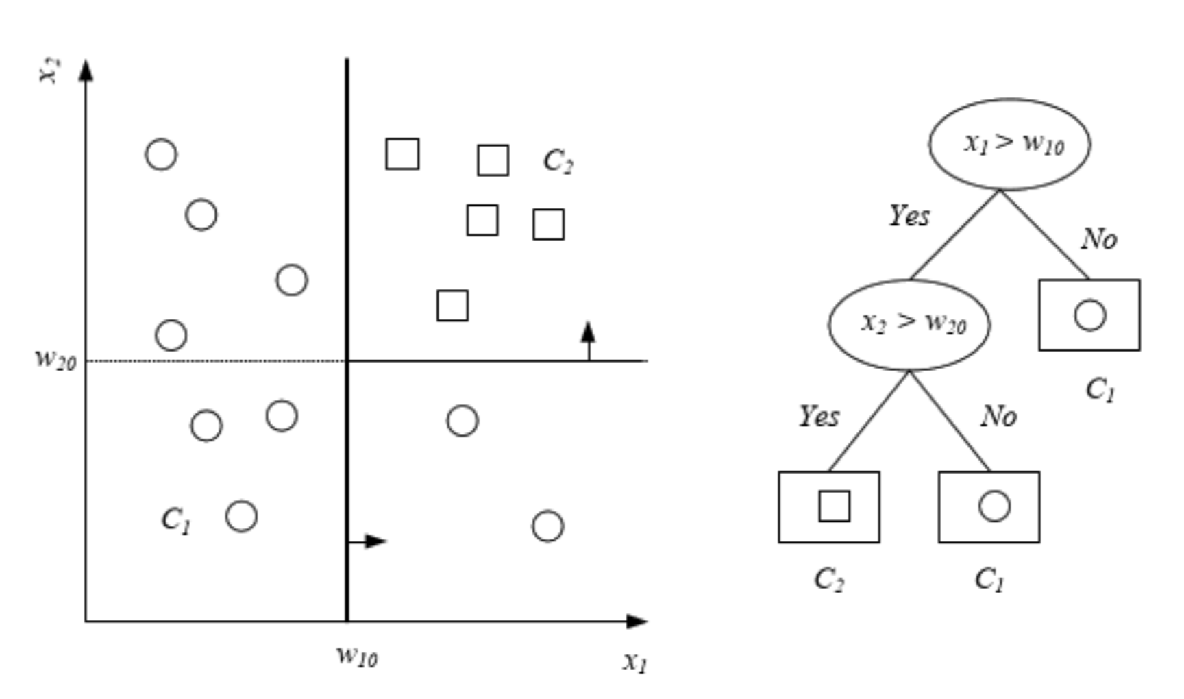
Decision tree is a hierarchical data structure that represents data through a divide and conquer strategy. They have a natural “if … then … else …” construction. It is a supervised learning algorithm (having a pre-defined target variable) that is used in classification and regression problems. It works for both categorical and continuous input and output variables. Decision Tree process starts at the root and is repeated recursively until a leaf node is hit (which are are more “pure” (i.e., homogeneous) in terms of the outcome variable), at which point the value written in the leaf constitutes the output.
A decision tree always considers all features and values for every feature. This means we could call it a greedy algorithm. The way a decision tree decides on which question, i.e. which feature, to ask, is by which question will have the highest information gain. In other words, it chooses the local optimal next feature. This process can be explained with three bullet points:
- Calculate impurity at root node
- Calculate information gain for each feature and value
- Choose the feature and values which grants the biggest information gain
One important thing to remember is that the decisions at the bottom of the tree are less statistically robust than those at the top because the decisions are based on less data.
Decision trees has three types of nodes. There is the root node, internal nodes and leaf nodes. However, you might also hear about other common terms, which are described below:
- Root Node: It represents entire population or sample and this further gets divided into two or more homogeneous sets. the only node without parents.
- Splitting: It is a process of dividing a node into two or more sub-nodes.
- Decision Node: When a sub-node splits into further sub-nodes, then it is called decision node.
- Leaf/ Terminal Node: Nodes do not split is called Leaf or Terminal node.
- Pruning: When we remove sub-nodes of a decision node, this process is called pruning. You can say opposite process of splitting.
- Branch / Sub-Tree: A sub section of entire tree is called branch or sub-tree.
- Parent and Child Node: A node, which is divided into sub-nodes is called parent node of sub-nodes whereas sub-nodes are the child of parent node.
- Depth of a tree is the maximal length of a path from the root node to a leaf node.
- Internal Node, each of which has exactly one incoming edge and two or more outgoing edges.

A Basic Example
Let’s just build a decision tree on iris dataset and take a look at how it makes predictions. The following code trains a DecisionTreeClassifier on the iris dataset!
from sklearn.datasets import load_iris
from sklearn.tree import DecisionTreeClassifier

iris = load_iris()
X = iris.data[:, 2:] # petal length and width
y = iris.target

tree_clf = DecisionTreeClassifier(max_depth=2, random_state=42)
tree_clf.fit(X, y)
# DecisionTreeClassifier(class_weight=None, criterion='gini', max_depth=2,
#                        max_features=None, max_leaf_nodes=None,
#                        min_impurity_decrease=0.0, min_impurity_split=None,
#                        min_samples_leaf=1, min_samples_split=2,
#                        min_weight_fraction_leaf=0.0, presort=False,
#                        random_state=42, splitter='best')
You can visualize the trained Decision Tree by first using the export_graphviz() method to output a graph definition file called iris_tree.dot:
from sklearn.tree import export_graphviz

export_graphviz(
        tree_clf,
        out_file="iris_tree.dot",
        feature_names=iris.feature_names[2:],
        class_names=iris.target_names,
        rounded=True,
        filled=True
    )
you can convert this .dot file to a variety of formats such as PDF or PNG using the dot command-line tool from graphviz package. The command line below converts the dot file to a png image file:
!dot -Tpng iris_tree.dot -o iris_tree.png
#This is a command on Terminal

# Or you can use the package pydot

import pydot
# Use dot file to create a graph
(graph, ) = pydot.graph_from_dot_file('iris_tree.dot')
# Write graph to a png file
graph.write_png('iris_tree_pydot.png')

# OR

from subprocess import call

call(['dot', '-T', 'png', 'iris_tree.dot', '-o', 'iris_tree_subprocess.png'])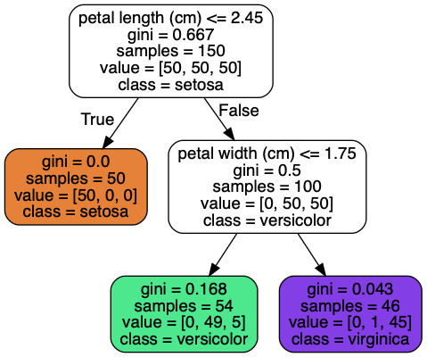
Making predictions
Suppose you find an iris flower and you want to classify it. You start at the root node (depth 0, at the top): this node asks whether the flower’s petal length is smaller than 2.45 cm. If it is, then you move down to the root’s left child node (depth 1, left). In this case, it is a leaf node (i.e., it does not have any children nodes), so it does not ask any questions: you can simply look at the predicted class for that node and the Decision Tree predicts that your flower is an Iris-Setosa (class=setosa).
Now suppose you find another flower, but this time the petal length is greater than 2.45 cm. You must move down to the root’s right child node (depth 1, right), which is not a leaf node, so it asks another question: is the petal width smaller than 1.75 cm? If it is, then your flower is most likely an Iris-Versicolor (depth 2, left). If not, it is likely an Iris-Virginica (depth 2, right). It’s really that simple.
tree_clf.predict([[5, 1.5]])
#array([1])
#Versicolor
How to interpret the tree above?
Root node:
samples = 150that means the node ‘contains’ 150 samples. Since it’s the root node that means the tree was trained on 150 samples.value = [50, 50, 50]are to give class probabilities. The data set contains 3 classes of 50 instances each (Iris Setosa, Iris Versicolour, Iris Virginica). About 1/3 of the samples belong to class Setosa and 1/3 to class Versicolour and 1/3 to Virginica.gini = 0.6667is the gini impurity of the node. It discribes how much the classes are mixed up. We compute it as follows: $1 - ((50/150)^{2} + (50/150)^{2} + (50/150)^{2}) = 0.6667$. Its formula is given below.petal length (cm) <= 2.45This means that the node is split so that all samples where the feature petal length (cm) is lower than 2.45 go to the left child and the samples where the feature is higher than 2.45 go to the right child.
A node’s samples attribute counts how many training instances it applies to. For example, 100 training instances have a petal length greater than 2.45 cm (depth 1, right), among which 54 have a petal width smaller than 1.75 cm (depth 2, left). A node’s value attribute tells you how many training instances of each class this node applies to: for example, the bottom-right node applies to 0 Iris-Setosa, 1 Iris- Versicolor, and 45 Iris-Virginica. Finally, a node’s gini attribute measures its impurity (Gini impurity is lower bounded by 0, with 0 occurring if the data set contains only one class): a node is “pure” (gini=0) if all training instances it applies to belong to the same class. For example, since the depth-1 left node applies only to Iris-Setosa training instances, it is pure and its gini score is 0. Equation below shows how the training algorithm computes the gini score $G_{i}$ of the $i$-th node. For example, the depth-2 left node has a gini score equal to $1 - (0/54)^{2} - (49/54)^{2} - (5/54)^{2} = 0.168$.
Considering we have $J$ classes, Gini index is computed by:
\begin{equation}
\begin{split}
I_{G} (p) &= \sum_{i=1}^{J} p_{i} \sum_{k \neq i} p_{k} = \sum_{i=1}^{J} p_{i} (1-p_{i})
&= \sum_{i=1}^{J} p_{i} - p_{i}^{2} = \sum_{i=1}^{J} p_{i} - \sum_{i=1}^{J} p_{i}^{2}
&= 1- \sum_{i=1}^{J} p_{i}^{2}
\end{split}
\end{equation}
This is for multiple classes and also used for binary classes.
For instance, if a data set has only one class, its gini index is $1 − 1^{2} = 0$, which is a purity data set. On the other hand, if a probability distribution is uniform $p = (1/k, 1/k, \cdots , 1/k)$, its gini index achieves maximum.
NOTE You might often come across the term ‘Gini Impurity’ which is determined by subtracting the gini value from 1. So mathematically we can say, $\text{Gini Impurity} = 1 - \text{Gini}$.
NOTE: Scikit-Learn uses the CART algorithm, which produces only binary trees and makes use of Gini impurity as metric to measure uncertainty: non-leaf nodes always have two children (i.e., questions only have yes/no answers). However, other algorithms such as Iterative Dichotomiser 3 (ID3) (and C4.5) which uses entropy as metric to measure uncertainty, can produce Decision Trees with nodes that have more than two children.
Estimating Class Probabilities
A Decision Tree can also estimate the probability that an instance belongs to a particular class k: first it traverses the tree to find the leaf node for this instance, and then it returns the ratio of training instances of class k in this node. For example, suppose you have found a flower whose petals are 5 cm long and 1.5 cm wide. The corresponding leaf node is the depth-2 left node, so the Decision Tree should output the following probabilities: 0% for Iris-Setosa (0/54 = 0), 90.7% for Iris-Versicolor (49/54 = 0.90740741), and 9.3% for Iris-Virginica (5/54 = 0.09259259). And of course if you ask it to predict the class, it should output Iris-Versicolor (class 1) since it has the highest probability.
tree_clf.predict_proba([[5, 1.5]])
#array([[0.        , 0.90740741, 0.09259259]])
The CART Training Algorithm
There are many methodologies for constructing decision trees but the most well-known is the classification and regression tree (CART) algorithm proposed in Breiman. CART uses binary recursive partitioning (it’s recursive because each split or rule depends on the the splits above it).
Scikit-Learn uses CART algorithm to train Decision Trees (also called “growing” trees). The idea is really quite simple: the algorithm first splits the training set in two subsets using a single feature $k$ and a threshold $t_{k}$ (e.g., “petal length $\leq$ 2.45”). How does it choose $k$ and $t_{k}$? It searches for the pair ($k, t_{k}$) that produces the purest subsets (weighted by their size). The cost function that the algorithm tries to minimize is then given by:
\begin{equation} J(k, t_{k}) = \frac{n_{left}}{n} G_{left} + \frac{n_{right}}{n} G_{right} \end{equation}
where $G_{left/right}$ measures the impurity of the left/right subset and $n_{left/right}$ is the number of instances in the left/right subset.

Once it has succesfully split the training set in two, it splits the subsets using the same logic, then the sub-subsets and so on, recursively. This process is continued until a suitable stopping criterion is reached (e.g., a maximum depth is reached or the tree becomes “too complex”). There are some other stopping conditions that we described below.
As one can see easily, the CART algorithm is a greedy algorithm. It greedily searches for an optimum split at the top level, then repeats the process at each level. It does not check whether or not the split will lead to the lowest possible impurity several levels down. A greedy algorithm often produces a resonably good solution, but it is not guaranteed to be the optimal solution.
It’s important to note that a single feature can be used multiple times in a tree. However, even when many features are available, a single feature may still dominate if it continues to provide the best split after each successive partition.
Gini Impurity or Entropy?
By default, the Gini impurity measure is used, but you can also select the entropy impurity measure instead by setting the criterion hyperparameter to “entropy”. The concept of entropy originated in thermodynamics as a measure of molecular disorder: entropy approaches zero when molecules are still and well ordered. It later spread to a wide variety of domains, including Shannon’s information theory, where it measures the average information content of a message (A reduction of entropy is often called an information gain): entropy is zero when all messages are identical. In Machine Learning, it is frequently used as an impurity measure: a set’s entropy is zero when it contains instances of only one class. Equation shows the definition of the entropy of the $i$th node. For example, the depth-2 left node in has an entropy equal to $-(49/54) * log_{2}(49/54) - (5/54) * log_{2}(5/54) \approx 0.4450$.
Considering $J$ is the number of classes in the set, entropy is calculated as:
\begin{equation} H_{i} = - \sum_{k=1}^{J} p_{k} log_{2}\left(p_{k} \right) \end{equation}
where $p_{k} \neq 0$.
So should you use Gini impurity or entropy? The truth is, most of the time it does not make a big difference: they lead to similar trees. Gini impurity is slightly faster to compute since you do not need to compute the log, so it is a good default. However, when they differ, Gini impurity tends to isolate the most frequent class in its own branch of the tree, while entropy tends to produce slightly more balanced trees.
Impurity - Entropy & Gini
Decision tree algorithms use information gain to split a node. There are three commonly used impurity measures used in binary decision trees: Entropy, Gini index, and Classification Error. A node having multiple classes is impure whereas a node having only one class is pure, meaning that there is no disorder in that node.
Entropy (Cross-Entropy) (a way to measure impurity):
\begin{equation} Entropy = - \sum_{j} p_{j} \log_{2} p_{j} \end{equation}
For two classes, the equation above is simplified into:
\[Entropy = - p \log_{2} (p) - q \log_{2} (q)\]where $p + q = 1$.
Gini index (a criterion to minimize the probability of misclassification):
\begin{equation} Gini = 1-\sum_{j} p_{j}^{2} \end{equation}
Classification Error:
\begin{equation} \text{Classification Error} = 1- \max p_{j} \end{equation}
where $p_{j}$ is the probability of class $j$.
The entropy is 0 if all samples of a node belong to the same class, and the entropy is maximal if we have a uniform class distribution. In other words, the entropy of a node (consist of single class) is zero because the probability is 1 and log (1) = 0. Entropy reaches maximum value when all classes in the node have equal probability.
-
Entropy of a group in which all examples belong to the same class: \begin{equation} entropy = -1 \log_2(1) = 0 \end{equation} This is not a good set for training.
-
entropy of a group with 50% in either class: \begin{equation} entropy = -0.5 \log_2 0.5 - 0.5 \log_2 0.5 = 1 \end{equation} This is a good set for training.
So, basically, the entropy attempts to maximize the mutual information (by constructing a equal probability node) in the decision tree.
Similar to entropy, the Gini index is maximal if the classes are perfectly mixed, for example, in a binary class:
\begin{equation} Gini = 1 - (p_1^2 + p_2^2) = 1-(0.5^2+0.5^2) = 0.5 \end{equation}
NOTE: Whether using gini or entropy, the resulting trees are typically very similar in practice. Maybe an advantage of Gini would be that you don’t need to compute the log, which can make it a bit faster in your implementation.
import matplotlib.pyplot as plt
%matplotlib inline
import numpy as np

def gini(p):
    return (p)*(1 - (p)) + (1 - p)*(1 - (1-p))

def entropy(p):
    return - p*np.log2(p) - (1 - p)*np.log2((1 - p))

def classification_error(p):
    return 1 - np.max([p, 1 - p])

x = np.arange(0.0, 1.0, 0.01)
ent = [entropy(p) if p != 0 else None for p in x]
scaled_ent = [e*0.5 if e else None for e in ent]
c_err = [classification_error(i) for i in x]

fig = plt.figure()
ax = plt.subplot(111)

for j, lab, ls, c, in zip(
      [ent, scaled_ent, gini(x), c_err],
      ['Entropy', 'Entropy (scaled)', 'Gini Impurity', 'Misclassification Error'],
      ['-', '-', '--', '-.'],
      ['lightgray', 'red', 'green', 'blue']):
   line = ax.plot(x, j, label=lab, linestyle=ls, lw=1, color=c)

ax.legend(loc='upper left', bbox_to_anchor=(0.01, 0.85),
         ncol=1, fancybox=True, shadow=False)

ax.axhline(y=0.5, linewidth=1, color='k', linestyle='--')
ax.axhline(y=1.0, linewidth=1, color='k', linestyle='--')

plt.ylim([0, 1.1])
plt.xlabel('p(j=1)')
plt.ylabel('Impurity Index')
plt.show()
Information Gain (IG)
Using a decision algorithm, we start at the tree root and split the data on the feature that maximizes information gain (IG). The Information Gain in Decision Tree is exactly the Standard Deviation Reduction we are looking to reach. We calculate by how much the Standard Deviation decreases after each split. Because the more the Standard Deviation is decreased after a split, the more homogeneous the child nodes will be. So the more homogeneous is your data in a part, the lower will be the entropy or gini impurity. The more you have splits, the more you have chance to find parts in which your data is homogeneous, and therefore the lower will be the entropy (close to 0) in these parts. However you might still find some nodes where the data is not homogeneous, and therefore the entropy would not be that small.
We repeat this splitting procedure at each child node down to the empty leaves. This means that the samples at each node all belong to the same class.
However, this can result in a very deep tree with many nodes, which can easily lead to overfitting. Thus, we typically want to prune the tree by setting a limit for the maximum depth of the tree.
Basically, using IG, we want to determine which attribute in a given set of training feature vectors is most useful. In other words, IG tells us how important a given attribute of the feature vectors is.
We will use it to decide the ordering of attributes in the nodes of a decision tree.
The Information Gain (IG) can be defined as follows:
\begin{equation} IG(G_p) = I(G_p) - \frac{n_{left}}{n}I(G_{left}) - \frac{n_{right}}{n}I(G_{right}) \end{equation}
where $I$ is impurity and could be entropy, Gini index, or classification error, $G_p$, $G_{left}$, and $G_{right}$ are the dataset of the parent, left and right child node. $n$ is the number of samples in the parent node. $n_{left}$ and $n_{right}$ are the number of samples are in the left child node and right child node respectively.
Information Gain (IG) - An Example
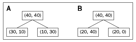
In this section, we’ll get IG for a specific case as shown below:
First, let’s use Classification Error to find the impurity in each node:
The impurity for parent node is then: \begin{equation} I_{CE}(G_p) = 1 - \frac{40}{80} = 1 - 0.5 = 0.5 \end{equation}
Let’s compute the impurity if we split by variable $A$: \begin{equation} A: I_{CE}(G_{left}) = 1 - \frac{30}{40} = 1 - \frac{3}{4} = 0.25 \end{equation}
\begin{equation} A: I_{CE}(G_{right}) = 1 - \frac{30}{40} = 1 - \frac{3}{4} = 0.25 \end{equation}
\begin{equation}
\begin{split}
IG_{A}(G_p) &= I_{CE}(G_p) - \frac{n_{left}}{n}I_{CE}(G_{left}) - \frac{n_{right}}{n}I_{CE}(G_{right})
&= 0.5 - \frac{40}{80} \times 0.25 - \frac{40}{80} \times 0.25 = 0.5 - 0.125 - 0.125
&= 0.25
\end{split}
\end{equation}
Similarly, let’s do all the calculations for variable $B$: \begin{equation} B:I_{CE}(G_{left}) = 1 - \frac{40}{60} = 1 - \frac{2}{3} = \frac{1}{3} \end{equation}
\begin{equation} B:I_{CE}(G_{right}) = 1 - \frac{20}{20} = 1 - 1 = 0 \end{equation}
\begin{equation}
\begin{split}
IG_{B}(G_p) &= I_{CE}(G_p) - \frac{n_{left}}{n}I_{CE}(G_{left}) - \frac{n_{right}}{n}I_{CE}(G_{right})
&= 0.5 - \frac{60}{80} \times \frac13 - \frac{20}{80} \times 0 = 0.5 - 0.25 - 0
&= 0.25
\end{split}
\end{equation}
The information gains using the classification error as a splitting criterion are the same (0.25) in both cases A and B.
Secondly, let’s use Gini index to find the impurity in each node:
The impurity for parent node is
\begin{equation} I_{Gini}(G_p) = 1 - \left( \left(\frac{40}{80} \right)^2 + \left(\frac{40}{80}\right)^2 \right) = 1 - (0.5^2+0.5^2) = 0.5 \end{equation}
Let’s compute the impurity if we split by variable $A$:
\begin{equation} A:I_{Gini}(G_{left}) = 1 - \left( \left(\frac{30}{40} \right)^2 + \left(\frac{10}{40}\right)^2 \right) = 1 - \left( \frac{9}{16} + \frac{1}{16} \right) = \frac38 = 0.375 \end{equation}
\begin{equation} A:I_{Gini}(G_{right}) = 1 - \left( \left(\frac{10}{40}\right)^2 + \left(\frac{30}{40}\right)^2 \right) = 1 - \left(\frac{1}{16}+\frac{9}{16}\right) = \frac38 = 0.375 \end{equation}
\begin{equation} IG_{A}(G_p) = 0.5 - \frac{40}{80} \times 0.375 - \frac{40}{80} \times 0.375 = 0.125 \end{equation}
Similarly, let’s do all the calculations for variable $B$:
\begin{equation} B:I_{Gini}(G_{left}) = 1 - \left( \left(\frac{20}{60} \right)^2 + \left(\frac{40}{60}\right)^2 \right) = 1 - \left( \frac{9}{16} + \frac{1}{16} \right) = 1 - \frac59 = 0.44 \end{equation}
\begin{equation} B:I_{Gini}(G_{right}) = 1 - \left( \left(\frac{20}{20}\right)^2 + \left(\frac{0}{20}\right)^2 \right) = 1 - (1+0) = 1 - 1 = 0 \end{equation}
\begin{equation} IG_{B}(G_p) = 0.5 - \frac{60}{80} \times 0.44 - 0 = 0.5 - 0.33 = 0.17 \end{equation}
So, the Gini index favors the split B.
Lastly, let’s use Entropy measure to find the impurity in each node:
The impurity for parent node is
\begin{equation} I_{Entropy}(G_p) = - \left( 0.5\log_2(0.5) + 0.5\log_2(0.5) \right) = 1 \end{equation}
Let’s compute the impurity if we split by variable $A$:
\begin{equation} A:I_{Entropy}(G_{left}) = - \left( \frac{30}{40}\log_2 \left(\frac{30}{40} \right) + \frac{10}{40}\log_2 \left(\frac{10}{40} \right) \right) = 0.81 \end{equation}
\begin{equation} A:I_{Entropy}(G_{right}) = - \left( \frac{10}{40}\log_2 \left(\frac{10}{40} \right) + \frac{30}{40}\log_2 \left(\frac{30}{40} \right) \right) = 0.81 \end{equation}
\begin{equation} IG_{A}(G_p) = 1 - \frac{40}{80} \times 0.81 - \frac{40}{80} \times 0.81 = 0.19 \end{equation}
Similarly, let’s do all the calculations for variable $B$:
\begin{equation} B:I_{Entropy}(G_{left}) = - \left( \frac{20}{60}\log_2 \left(\frac{20}{60} \right) + \frac{40}{60}\log_2 \left(\frac{40}{60} \right) \right) = 0.92 \end{equation}
\begin{equation} B:I_{Entropy}(G_{right}) = - \left( \frac{20}{20}\log_2 \left(\frac{20}{20} \right) + 0 \right) = 0 \end{equation}
\begin{equation} IG_{B}(G_p) = 1 - \frac{60}{80} \times 0.92 - \frac{20}{80} \times 0 = 0.31 \end{equation}
So, the entropy criterion favors B.
How to split with different variable?
The set of split points considered for any variable depends upon whether the variable is numeric or categorical (nominal/ordinal). Splits can be multi-way (for example, for the variable “size” - Small/Medium/Large) or binary (for example, for the variable “Taxable Income > 80K?” - Yes/No). Binary split can also divide values into two subsets, for example, for the variable “size”, we can consider {Small, Medium}/Large OR {Medium, Large}/Small, OR {Small, Large}/Medium
When a predictor is numerical, we can use a brute-force method to split this variable to use a Decision Tree algorithm. If all values are unique, there are $n - 1$ split points for $n$ data points. Suppose we have a training set with an attribute “age” which contains following values: 10, 11, 16, 18, 20, 35. Now at a node, the algorithm will consider following possible splitting:
\[\begin{split} Age \leq 10 \quad & \quad Age>10 \\ Age \leq 11 \quad & \quad Age>11 \\ Age \leq 16 \quad & \quad Age>16 \\ Age \leq 18 \quad & \quad Age>18 \\ Age \leq 20 \quad & \quad Age>20 \\ Age \leq 35 \quad & \quad Age>35 \\ \end{split}\]At every split candidate, we then compute the Gini index and choose the that gives the lowest value. However, this approach is computationally expensive because we need to consider every value of the attribute in the N records as a candidate split position.
Because number of unique values of a numerical attribute may be a large number, it is common to consider only split points at certain percentiles of the distribution of values. For example, we may consider every tenth percentile (that is, 10%, 20%, 30%, etc).
Another way to do so is to discretize the values into ranges and treat this numerical attribute as a categorical variable.
Alternatively, we can split nodes based on thresholds ($A < c$) such that the data is partitioned into examples that satisfy $A < c$ and $A \geq c$. Information gain for these splits can be calculated in the same way as before, since in this setup each node becomes a Boolean value. To find the split with the highest gain for continuous attribute A, we would sort examples according to the value, and for each ordered pair (x, y) with different labels, we would check the midpoint as a possible threshold. For example, consider the following data:
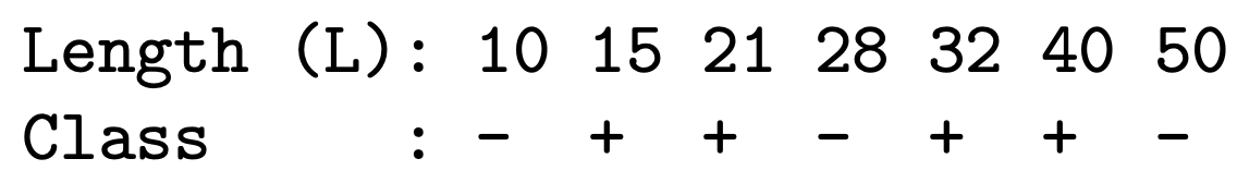
Using the above, we would check thresholds $L < 12.5$, $L < 24.5$, $L < 45$, and could then use the standard decision tree algorithms. It is important to note, though, that domain knowledge may influence how we choose these splits; the midpoint may not always be appropriate (for example for the variable ‘age’. We won’t consider $Age \leq 10.5$ as 10.5 never appears in the training set)
When a predictor is categorical we can decide to split it to create either one child node per class (multi-way splits) or only two child nodes (binary split). It is usual to make only binary splits because multiway splits break the data into small subsets too quickly. This causes a bias towards splitting predictors with many classes since they are more likely to produce relatively pure child nodes, which results in overfitting.
If a categorical predictor has only two classes, there is only one possible split. However, if a categorical predictor has more than two classes, various conditions can apply.
If there is a small number of classes, all possible splits into two child nodes can be considered.
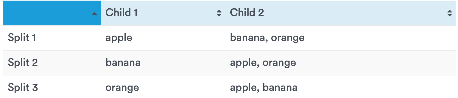
For $k$ classes there are $2^{k-1} – 1$ splits, which is computationally prohibitive if $k$ is a large number.
Ordinal attributes can also produce binary or multi-way splits. Ordinal attribute values can be grouped as long as the grouping does not violate the order property of the attribute values.
If there are many classes, they may be ordered according to their average output value. We can the make a binary split into two groups of the ordered classes. This means there are $k – 1$ possible splits for $k$ classes.
If $k$ is large, there are more splits to consider. As a result, there is a greater chance that a certain split will create a significant improvement, and is therefore best. This causes trees to be biased towards splitting variables with many classes over those with fewer classes.
Regularization Hyperparameters
Decision Trees make very few assumptions about the training data (as opposed to linear models, which obviously assume that the data is linear, for example). If left unconstrained, the tree structure will adapt itself to the training data, fitting it very closely, and most likely overfitting it. Such a model is often called a nonparametric model, not because it does not have any parameters (it often has a lot) but because the number of parameters is not determined prior to training, so the model structure is free to stick closely to the data. In contrast, a parametric model such as a linear model has a predetermined number of parameters, so its degree of freedom is limited, reducing the risk of overfitting (but increasing the risk of underfitting).
To avoid overfitting the training data, you need to restrict the Decision Tree’s freedom during training. As you know by now, this is called regularization.
The DecisionTreeClassifier of Scikit-Learn package class has a few parameters that similarly restrict the shape of the Decision Tree. Increasing min_* hyperparameters or reducing max_* hyperparameters will regularize the model.
-
Maximum number of terminal nodes
max_leaf_nodes: The maximum number of terminal nodes or leaves in a tree. can be defined in place of max_depth. Since binary trees are created, a depth of $n$ would produce a maximum of $2^n$ leaves. -
Maximum features that are evaluated for splitting at each node
max_features: The number of features to consider while searching for a best split. These will be randomly selected. As a thumb-rule, square root of the total number of features works great but we should check upto 30-40% of the total number of features. Higher values can lead to over-fitting but depends on case to case. -
Minimum samples for a node split
min_samples_split: Defines the minimum number of samples (or observations) which are required, a node must have before it can be split. Used to control over-fitting. Higher values prevent a model from learning relations which might be highly specific to the particular sample selected for a tree. Too high values can lead to under-fitting hence, it should be tuned using CV. -
Minimum samples for a terminal node (leaf)
min_samples_leaf: Defines the minimum samples (or observations) required in a terminal node or leaf. Used to control over-fitting similar to min_samples_split. Generally lower values should be chosen for imbalanced class problems because the regions in which the minority class will be in majority will be very small. Similarly,min_weight_fraction_leaf(same as min_samples_leaf but expressed as a fraction of the total number of weighted instances). -
Maximum depth of tree (vertical depth)
max_depth: The maximum depth of a tree. Used to control over-fitting as higher depth will allow model to learn relations very specific to a particular sample. Should be tuned using CV. Reducingmax_depthwill regularize the model and thus reduce the risk of overfitting. The default value inDecisionTreeClassifierof Scikit-Learn package isNone, which means unlimited.
What is the optimal Tree Depth?
We need to be careful to pick an appropriate tree depth. If the tree is too deep, we can overfit. If the tree is too shallow, we underfit. Max depth is a hyper-parameter that should be tuned by the data. Alternative strategy is to create a very deep tree, and then to prune it.
A node whose children are all leaf nodes is considered unnecessary if the purity improvement it provides is not statistically significant. Standard statistical tests, such as the $\chi^{2}$ test, are used to estimate the probability that the improvement is purely the result of chance (which is called the null hypothesis). If this probability, called the p-value, is higher than a given threshold (typically 5%, controlled by a hyperparameter), then the node is considered unnecessary and its children are deleted. The pruning continues until all unnecessary nodes have been pruned.
Regression
Decision Tree are also capable of performing regression tasks. Let’s build a regression tree using Scikit’s Learn DecisionTreeRegressor class, training it on a noisy quadratic dataset with max_depth =2:
import numpy as np
# Quadratic training set + noise
np.random.seed(42)
m = 200
X = np.random.rand(m, 1)
y = 4 * (X - 0.5) ** 2
y = y + np.random.randn(m, 1) / 10
from sklearn.tree import DecisionTreeRegressor
tree_reg = DecisionTreeRegressor(max_depth=2, random_state=42)
tree_reg.fit(X, y)
# DecisionTreeRegressor(criterion='mse', max_depth=2, max_features=None,
# max_leaf_nodes=None, min_impurity_decrease=0.0,
# min_impurity_split=None, min_samples_leaf=1,
# min_samples_split=2, min_weight_fraction_leaf=0.0,
# presort=False, random_state=42, splitter='best')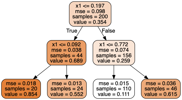
This tree looks very similar to the classification tree you built earlier. The main difference is that instead of predicting a class in each node, it predicts a value. For example, suppose you want to make a prediction for a new instance with $x1 = 0.6$. You traverse the tree starting at the root, and you eventually reach the leaf node that predicts $value=0.111$. This prediction is simply the average target value of the 110 training instances associated to this leaf node. This prediction results in a Mean Squared Error (MSE) equal to $0.0151$ over these 110 instances.
The CART algorithm works mostly the same way as earlier, except that instead of trying to split the training set in a way that minimizes impurity, it now tries to split the training set in a way that minimizes the MSE. Equation shows the cost function that the algorithm tries to minimize.
\begin{equation} J(k, t_{k}) = \frac{n_{left}}{n} MSE_{left} + \frac{n_{right}}{n} MSE_{right} \end{equation}
where $MSE_{left/right}$ measures the impurity of the left/right subset and $n_{left/right}$ is the number of instances in the left/right subset.
\begin{equation} MSE_{node} = \sum_{i \in node} \left(\hat{y}_{node} - y^{(i)}\right)^{2} \end{equation}
and
\[\hat{y}_{node} = \frac{1}{n_{node}} \sum_{i \in node} y^{(i)}\]Just like for classification tasks, Decision Trees are prone to overfitting when dealing with regression tasks.
Differences and Similarities Between Regression and Classification Trees
- Regression trees are used when dependent variable is continuous. Classification trees are used when dependent variable is categorical.
- In case of regression tree, the value obtained by terminal nodes in the training data is the mean response of observation falling in that region. Thus, if an unseen data observation falls in that region, we’ll make its prediction with mean value.
- In case of classification tree, the value (class) obtained by terminal node in the training data is the mode of observations falling in that region. Thus, if an unseen data observation falls in that region, we’ll make its prediction with mode value.
- Both the trees divide the predictor space (independent variables) into distinct and non-overlapping regions. For the sake of simplicity, you can think of these regions as high dimensional boxes or boxes.
- Both the trees follow a top-down greedy approach known as recursive binary splitting. We call it as ‘top-down’ because it begins from the top of tree when all the observations are available in a single region and successively splits the predictor space into two new branches down the tree. It is known as ‘greedy’ because, the algorithm cares (looks for best variable available) about only the current split, and not about future splits which will lead to a better tree.
- This splitting process is continued until a user defined stopping criteria is reached. For example: we can tell the the algorithm to stop once the number of observations per node becomes less than 50.
- In both the cases, the splitting process results in fully grown trees until the stopping criteria is reached. But, the fully grown tree is likely to overfit data, leading to poor accuracy on unseen data. This bring ‘pruning’. Pruning is one of the technique used tackle overfitting.
How should the splitting procedure stop?
A stopping condition is needed to terminate the tree growing process. The basic version of the decision tree algorithm keeps subdividing tree nodes until every leaf is pure (when all the records belong to the same class). Another strategy is to continue expanding a node until all the records have identical attribute values. Although both conditions are sufficient to stop any decision tree induction algorithm, other early termination criteria can be imposed to allow the tree-growing procedure to terminate earlier.
Pruning Trees
While stopping criteria are a relatively crude method of stopping tree growth, early studies showed that they tended to degrade the tree’s performance. An alternative approach to stopping growth is to allow the tree to grow and then prune it back to an optimum size.
Frequently, a node is not split further if the number of training instances reaching a node is smaller than a certain percentage of the training set (Minimum samples for a terminal node (leaf)), for example 5 percent, regardless of impurity or error. The idea is that any decision based on too few instances can cause the variance and thus generalization error. Stopping tree construction early on before it is full is called preprunning the tree (also known as Early Stopping Rule).
Another possibility to get simpler trees is postpruning, which in practice works better than preprunning. Tree growing is greedy and at each step, we can a decision, namely to generate a decision node and continue to further on, never backtracking, and trying out an altervative. The only exception is postprunning where we try to find and prune unnecessary subtrees.
Any pruning should reduce the size of a learning tree without reducing predictive accuracy as measured by a cross-validation set.
Comparing preprunning and postprunning, we can say that preprunning is faster but postprunning generally leads to more accurate trees.
Advantages
-
Easy to understand, interpret, visualize.: Decision tree is a white-box model and its output is very easy to understand even for people from non-analytical background. It does not require any statistical knowledge to read and interpret them. Its graphical representation is very intuitive and users can easily relate their hypothesis (if the trees are small).
-
They perform internal feature selection or variable screening as an integral part of the procedure. They are thereby resistant, if not completely immune, to the inclusion of many irrelevant predictor variables.
-
Less data cleaning required: It requires less data cleaning compared to some other modeling techniques. It is not influenced by outliers and missing values to a fair degree. For classification, most likely outliers will have a negligible effect because the nodes are determined based on the class proportions in each split region. In other words, after a node splits the data into two groups you only need to know the labels (or their counts) in each group to determine how good the split is (the outlier in the input variable has no influence on the calculation. They do a slice on the data, and then after that slice, it doesn’t matter how big of a value you have. If you had five data points, and one of their features looked like ${1,2,3,4,1,000,000}$ , you might choose a split point at $x = 2.5$. At that point, 3, 4, and a million all go into the same bucket, and their values are treated the same way. You could replace one million with something orders of magnitude bigger and it wouldn’t matter, or you could change its value to 5 and it wouldn’t matter. For the regression case, we use variance reduction (MSE) to find the optimal split, by minimizing MSE in each of the resulting regions. Therefore, if the technique used for splitting is variance reduction then while calculating the variance/standard deviation of two splitted groups(child nodes) vs the non-splitted group(parent node) outliers in the TARGET variable will have influence. BE CAREFUL! the variance refers to the variance in the target variable, not the inputs.
-
Decision Trees can naturally handle both numerical and categorical variables. Can also handle multi-output problems.
-
Decision tree is considered to be a non-parametric method. This means that decision trees have no assumptions about the space distribution and the classifier structure.
-
Non-linear relationships between parameters do not affect tree performance.
-
The number of hyper-parameters to be tuned is almost null.
-
Decision Trees can handle multicollinearity. They make no assumptions on relationships between features. They are greedy algorithms. They will fit on the most effective variable they encounter, leaving other plausible variables out. It just constructs splits on single features that improves classification, based on an impurity measure like Gini or entropy. If features A, B are heavily correlated, no /little information can be gained from splitting on B after having split on A. So it would typically get ignored in favor of C.
Disadvantages
-
Decision-tree learners can create over-complex trees that do not generalize the data well. This is called overfitting. This problem gets solved by setting constraints on model parameters (e.g., limiting depth of the tree) and heavily pruning.
-
Not fit for continuous variables: While working with continuous numerical variables, decision tree loses information, when it categorizes variables in different categories.
-
Decision trees can be unstable because small variations in the data might result in a completely different tree being generated. This is called variance, which needs to be lowered by methods like bagging and boosting.
-
Greedy algorithm, which always makes the choice that seems to be the best at that moment without regard for consequences, cannot guarantee to return the globally optimal decision tree. This is its over–sensitivity to the training set, to irrelevant attributes and to noise. This can be mitigated by training multiple trees, where the features and samples are randomly sampled with replacement (Random Forest).
-
Decision tree learners create biased trees if some classes dominate. It is therefore recommended to balance the data set prior to fitting with the decision tree.
-
Calculations can become complex when there are many class labels.
-
Generally, it gives low prediction accuracy for a dataset as compared to other machine learning algorithms.
-
Information gain in a decision tree with categorical variables gives a biased response for attributes with greater number of categories.
-
It cannot be used for incremental learning (online learning).
-
Decision trees also suffer from the curse of dimensionality. Decision trees directly partition the sample space at each node. As the sample space increases, the distances between data points increases, which makes it much harder to find a “good” split.
-
Decision Tree cannot extrapolate outside of the range of variables.
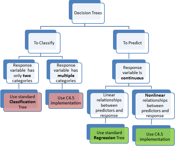
Types of Decision Tree
An Exercise
Train and fine-tune a Decision Tree for the moons dataset.
- Generate a moons dataset using make_moons(n_samples=10000, noise=0.4).
- Split it into a training set and a test set using train_test_split().
- Use grid search with cross-validation (with the help of the
GridSearchCVclass) to find good hyperparameter values for aDecisionTreeClassifier. Hint: try various values formax_leaf_nodes. - Train it on the full training set using these hyperparameters, and measure your model’s performance on the test set. You should get roughly 85% to 87% accuracy.
from sklearn.datasets import make_moons
from sklearn.model_selection import train_test_split
from sklearn.model_selection import GridSearchCV
from sklearn.metrics import accuracy_score

X, y = make_moons(n_samples=10000, noise=0.4, random_state=42)
X_train, X_test, y_train, y_test = train_test_split(X, y, test_size=0.2, random_state=42)

params = {'max_leaf_nodes': list(range(2, 100)), 'min_samples_split': [2, 3, 4]}
grid_search_cv = GridSearchCV(DecisionTreeClassifier(random_state=42), params, n_jobs=-1, verbose=1, cv=3, refit=True)

grid_search_cv.fit(X_train, y_train)

grid_search_cv.best_estimator_

# By default, GridSearchCV trains the best model found on the whole training set (you can change this by setting refit=False),
#so we don't need to do it again. We can simply evaluate the model's accuracy:
y_pred = grid_search_cv.predict(X_test)
accuracy_score(y_test, y_pred)
#0.8695
Differences between Random Forest and Decision Tree
Random Forest is a collection of Decision Trees. Decision Tree makes its final decision based on the output of one tree but Random Forest combines the output of a large number of small trees while making its final prediction. Following is the detailed list of differences between Decision Tree and Random Forest:
-
Random Forest is an Ensemble Learning (Bagging) Technique unlike Decision Tree: In Decision Tree, only one tree is grown using all the features and observations. But in case of Random Forest, features and observations are splitted into multiple parts and a lot of small trees (instead of one big tree) are grown based on the splitted data. So, instead of one full tree like Decision Tree, Random Forest uses multiple trees. Larger the number of trees, better is the accuracy and generalization capability. But at some point, increasing the number of trees does not contribute to the accuracy, so one should stop growing trees at that point.
-
Random Forest uses voting system unlike Decision Tree: All the trees grown in Random Forest are called weak learners. Each weak learner casts a vote as per its prediction. The class which gets maximum votes is considered as the final output of the prediction. You can think of it like a democracy system. On the other hand, there is no voting system in Decision Tree. Only one tree predicts the outcome. No democracy at all!!
-
Random Forest rarely overfits unlike Decision Tree: Decision Tree is very much prone to overfitting as there is only one tree which is responsible for predicting the outcome. If there is a lot of noise in the dataset, it will start considering the noise while creating the model and will lead to very low bias (or no bias at all). Due to this, it will show a lot of variance in the final predictions in real world data. This scenario is called overfitting. In Random Forest, noise has very little role in spoiling the model as there are so many trees in it and noise cannot affect all the trees.
-
Random Forest reduces variance instead of bias: Random forest reduces variance part of the error rather than bias part, so on a given training dataset, Decision Tree may be more accurate than a Random Forest. But on an unexpected validation dataset, Random Forest always wins in terms of accuracy.
-
The downside of Random Forest is that it can be slow if you have a single process but it can be parallelized.
-
Decision Tree is easier to understand and interpret: Decision Tree is simple and easy to interpret. You know what variable and what value of that variable is used to split the data and predict the outcome. On the other hand, Random Forest is like a Black Box. You can specify the number of trees you want in your forest (
n_estimators) and also you can specify maximum number of features to be used in each tree. But you cannot control the randomness, you cannot control which feature is part of which tree in the forest, you cannot control which data point is part of which tree.