Ensemble Learning in extensive details with examples in Scikit-Learn

Bootstrap Method

This statistical technique consists in generating samples (called bootstrap samples) from an initial dataset of size N by randomly drawing with replacement (meaning we can select the same value multiple times)..

In bootstrap sampling, some original examples may appear more than once and some original examples are not present in the sample. If you want to create a sub-dataset with m elements, you should select a random element from the original dataset m times. And if the goal is generating n dataset, you follow this step n times. At the end, we have n datasets where the number of elements in each dataset is m.

Ensemble Learning

If you aggregate the predictions of a group of predictors (such as classifiers and regressors), you will often get better predictions than the best individual predictor. A group of predictors is called an ensemble, thus, this technique is called Ensemble Learning, and an Ensemble Learning algorithm is called an Ensemble method. They can be seen as a type of meta-algorithms, in the sense that they are methods composed of other methods.

Most ensemble methods use a single base learning algorithm to produce homogeneous base learners, i.e. learners of the same type, leading to homogeneous ensembles.

There are also some methods that use heterogeneous learners, i.e. learners of different types, leading to heterogeneous ensembles. In order for ensemble methods to be more accurate than any of its individual members, the base learners have to be as accurate as possible and as diverse as possible.

If we choose base models with low bias but high variance, it should be with an aggregating method that tends to reduce variance whereas if we choose base models with low variance but high bias, it should be with an aggregating method that tends to reduce bias.

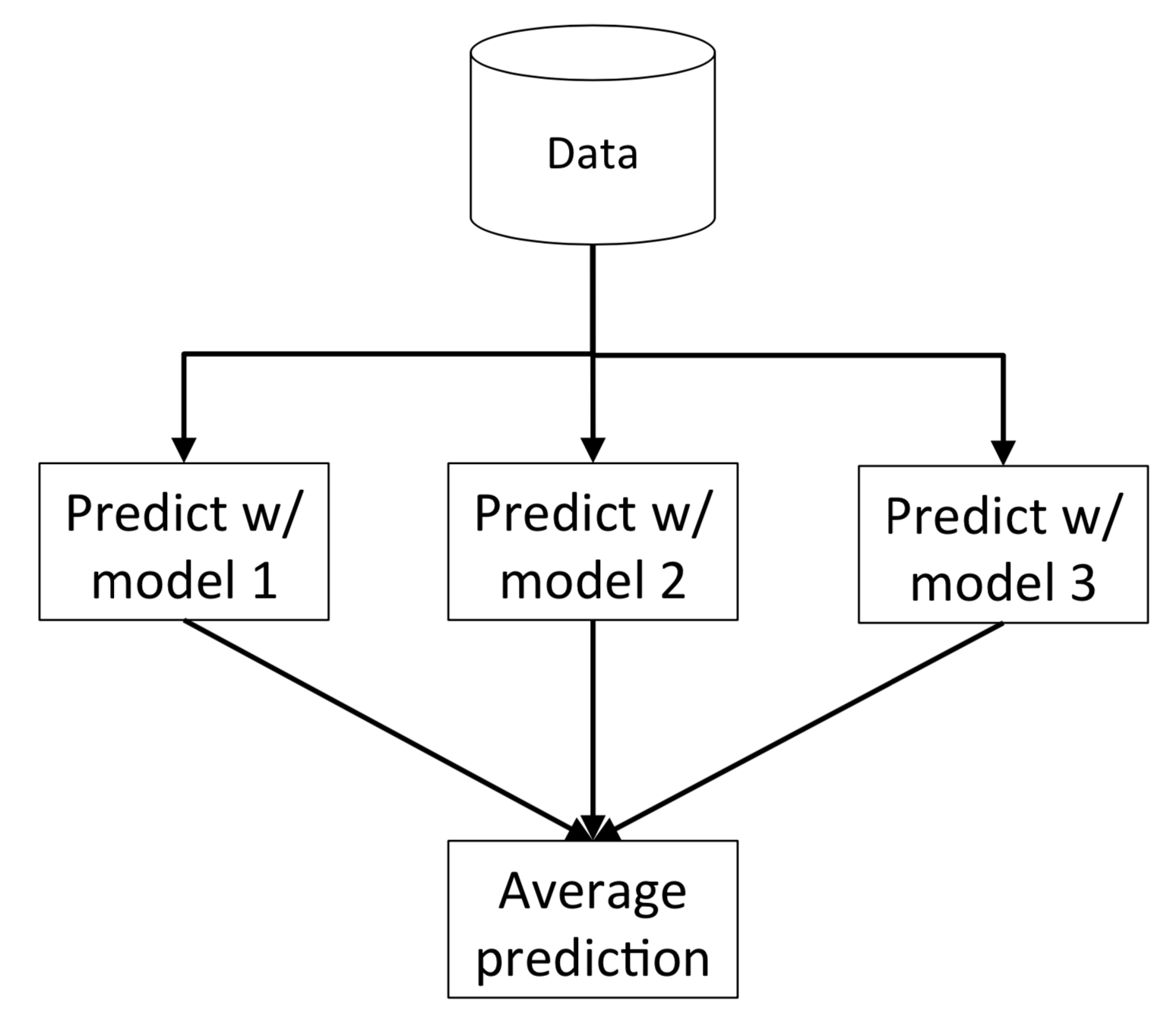
Voting and Averaging Based Ensemble Methods

Voting and averaging are two of the easiest ensemble methods. They are both easy to understand and implement. Voting is used for classification and averaging is used for regression.

In both methods, the first step is to create multiple classification/regression models using some training dataset. Each base model can be created using different splits of the same training dataset and same algorithm, or using the same dataset with different algorithms, or any other method.

In this method, we create predictions for each model and saved them in a matrix called predictions where each column contains predictions from one model.

1. Majority Voting (Hard voting)

   Every model makes a prediction (votes) for each test instance and the final output prediction. A hard voting classifier just counts the votes of each classifier in the ensemble and picks the class that gets the most votes. In some articles, you may see this method being called “plurality voting”. For example, assuming that we combine three classifiers that classify a training sample as follows: classifier 1 -> class 0, classifier 2 -> class 0, classifier 3 -> class 1. Via majority vote, we would we would classify the sample as “class 0.

   A soft voting classifier computes the average estimated class probability for each class and the picks the class with the highest probability. It only works only if every classifier is able to estimate class probabilities (i.e., they all have predict_proba() method). Assuming the example in the previous section was a binary classification task with class labels ${0,1}$, our 3-classifers ensemble could make the following prediction: $p_1(\mathbf{x}) \rightarrow [0.9, 0.1]$, $p_2(\mathbf{x}) \rightarrow [0.8, 0.2]$ and $p_3(\mathbf{x}) \rightarrow [0.4, 0.6]$. Using uniform weights, we compute the average probabilities: $p(Class = 0 \mid \mathbf{x}) = \frac{0.9 + 0.8 + 0.4}{3} = 0.7$ and $p(Class = 1 \mid \mathbf{x}) = \frac{0.1 + 0.2 + 0.6}{3} = 0.3$. Therefore, $\hat{y} = \arg \max \big[p(Class = 0 \mid \mathbf{x}), p(Class = 1 \mid \mathbf{x}) \big] = 0$

   Note that its also possible to introduce a weight vector to give more or less importance to each classifier.

2. Weighted Voting

   Unlike majority voting, where each model has the same rights, we can increase the importance of one or more models. In weighted voting you count the prediction of the better models multiple times. Finding a reasonable set of weights is up to you.

3. Simple Averaging

   In simple averaging method, for every instance of test dataset, the average predictions are calculated. This method often reduces overfit and creates a smoother regression model.

4. Weighted Averaging

   Weighted averaging is a slightly modified version of simple averaging, where the prediction of each model is multiplied by the weight and then their average is calculated

Note: The accuracy of the VotingClassifier is generally higher than the individual classifiers. Make sure to include diverse classifiers so that models which fall prey to similar types of errors do not aggregate the errors.

Bootstrap Aggregation (Bagging) And Pasting

Bootstrap Aggregation (or Bagging for short, also called Parallel Ensemble), is a simple and very powerful ensemble method. Ensembles are combinations of multiple diverse (potentially weak) models trained on a different set of datasets and almost always outperform the best model in the ensemble. It aims at producing an ensemble model that is more robust than the individual models composing it. The basic motivation of parallel methods is to exploit independence between the base learners since the error can possibly be reduced dramatically by averaging.

Specifically, bagging involves constructing k different datasets. Each dataset has the same number of examples as the original dataset, but each dataset is contructed by sampling with replacement. This means that, with high probability, each dataset is missing some of the examples from the original dataset and contains several duplicate examples (on average around two-thirds of the examples from the original dataset are found in the resulting training set, if it has the same size as the original). Model i is then trained on dataset i. The differences between which examples are included in each dataset results in differences between the trained models.

NOTE: It is a general procedure that can be used to reduce the variance for those algorithm that have high variance such as decision trees, like Classification And Regression Trees (CART) (Ensembling can reduce variance without increasing bias. It is however, only helpful if bias is low).

A bootstrap sample is created with sampling with replacement, and is of equal size as the original sample. It is a method of data perturbation and diversity generation. Because trees are very sensitive to small changes in the data, building multiple trees and averaging the predictions can yield drastic improvements in predictive performance

When sampling is performed without replacement, it is called pasting.

Both bagging and pasting allow training instances to be sampled several times across multiple predictors but only bagging allows training instances to be sampled several times for the same predictor.

How does Bagging work?

Let’s assume we have a sample dataset of 1000 instances (x) and we are using the CART algorithm (it can, as well, be different algorithms). Bagging of the CART algorithm would work as follows.

1. Create many (e.g. 100) random sub-samples of our dataset with replacement (or no replacement).
2. Train a CART model on each sample (The models run in parallel and are perfectly independent of each other and making uncorrelated errors).
3. The final predictions are determined by combining the predictions from all the models (Just like the decision trees themselves, Bagging can be used for classification and regression problems. The final predictions are obtained generally calculating the average prediction from each model for regression problem and simple majority vote for classification problem).

For example, if we had 5 bagged decision trees that made the following class predictions for a in input sample: blue, blue, red, blue and red, we would take the most frequent class and predict blue.

For classification problem the class outputted by each model can be seen as a vote and the class that receives the majority of the votes is returned by the ensemble model (this is called hard-voting). Still for a classification problem, we can also consider the probabilities of each classes returned by all the models, average these probabilities and keep the class with the highest average probability (this is called soft-voting). Averages or votes can either be simple or weighted if any relevant weights can be used.

Idea of bagging comes from the fact that averaging models reduces model variance. Since trees are notoriously noisy, they benefit greatly from the averaging. Moreover, since each tree generated in bagging is identically distributed (i.d.), the expectation of an average of $B$ such trees is the same as the expectation of any one of them. This means the bias of bagged trees is the same as that of the individual trees, and the only hope of improvement is through variance reduction. This is in contrast to boosting, where the trees are grown in an adaptive way to remove bias, and hence are not i.d.

An average of $B$ identically distributed (but possible dependent) random variables $\frac{1}{B}\sum_{i=1}^{B} X_{i}$, each with mean $\mu$ and variance $\sigma^{2}$, has mean $\mu$ variance $\frac{1}{B}\sigma^{2}$. If the variables are simply i.d. (identically distributed, but not necessarily independent) with positive pairwise correlation $\rho$, the variance of the average is computed as follows:

Suppose, in the above summation, that $i=j$. Then $\text{Cov}(X_i, X_j) = \sigma^2$. Exactly 𝐵 of these occur.

Suppose, in the above summation, that $i \neq j$. Then $\text{Cov}(X_i, X_j) = \rho\sigma^2$, since $\rho (X_i, X_j) = \frac{\text{Cov}(X_i, X_j)}{\sqrt{Var(X_{i}) Var(X_{j})}}$ where the variances are identical. There are $B^2 - B = B(B-1)$ of these occurrences. Hence,

As $B$ increases, the second term disappears (or can be made arbitrarily small), but the first term remains, and hence the size of the correlation of pairs of bagged trees limits the benefits of averaging. This is where the idea of random forest, which is to improve the variance reduction of bagging by reducing the correlation between the trees, without increasing the variance too much, comes in which we will talk a bit later. But until then, let’s stick to bagging… Also note that the bias of prediction model is tightly connected to its mean value. Consequently, by averaging the predictions from several identically distributed models, each with low bias, the bias remains low and the variance is reduced. This is achieved in the tree-growing process through random selection of the input variables which we will see in the next part.

When bagging with decision trees, we are less concerned about individual trees overfitting the training data. For this reason and for efficiency, the individual decision trees are grown deep (e.g. few training samples at each leaf-node of the tree) and the trees are not pruned. These trees will have both high variance and low bias. These are important characterize of sub-models when combining predictions using bagging.

The only parameters when bagging decision trees is the number of samples and hence the number of trees to include. This can be chosen by increasing the number of trees on run after run until the accuracy begins to stop showing improvement (e.g. on a cross validation test harness). Very large numbers of models may take a long time to prepare, but will not overfit the training data.

Recall that bagging typically results in improved accuracy over prediction using a single tree. Unfortunately, however, it can be difficult to interpret the resulting model. Thus, bagging improves prediction accuracy at the expense of interpretability

Random Forest is another ensemble machine learning algorithm that follows the bagging technique.

Classifying a dataset with a voting classifier

import numpy as np
import pandas as pd
import matplotlib.pyplot as plt
%matplotlib inline

from sklearn.model_selection import train_test_split
from sklearn.datasets import make_moons

X, y = make_moons(n_samples=500, noise=0.30, random_state=42)
X_train, X_test, y_train, y_test = train_test_split(X, y, random_state=42)

Classifying with hard voting

from sklearn.ensemble import RandomForestClassifier
from sklearn.ensemble import VotingClassifier
from sklearn.naive_bayes import GaussianNB
from sklearn.linear_model import LogisticRegression
from sklearn.svm import SVC
from sklearn.metrics import confusion_matrix

#voting classifier contains different classifier methods. Here, we'll create a set of classifiers.
log_clf = LogisticRegression(solver="liblinear", random_state=42)
gnb_clf = GaussianNB()
rnd_clf = RandomForestClassifier(n_estimators=10, random_state=42)
svm_clf = SVC(gamma="auto", random_state=42)

#Next, we'll create VoitngClassifier model with base classifier methods.
voting_clf = VotingClassifier(
    estimators=[('lr', log_clf), ('rf', rnd_clf), ('svc', svm_clf), ('gnb', gnb_clf)],
    voting='hard')

voting_clf.fit(X_train, y_train)

from sklearn.metrics import accuracy_score

for clf in (log_clf, rnd_clf, svm_clf, gnb_clf, voting_clf):
    clf.fit(X_train, y_train)
    y_pred = clf.predict(X_test)
    print(clf.__class__.__name__, accuracy_score(y_test, y_pred))
    print('Confusion Matrix for {}'.format(clf.__class__.__name__))
    print(confusion_matrix(y_test, y_pred ))
    print('\n')
    
# LogisticRegression 0.864
# Confusion Matrix for LogisticRegression
# [[56  5]
#  [12 52]]


# RandomForestClassifier 0.872
# Confusion Matrix for RandomForestClassifier
# [[59  2]
#  [14 50]]


# SVC 0.888
# Confusion Matrix for SVC
# [[60  1]
#  [13 51]]


# GaussianNB 0.856
# Confusion Matrix for GaussianNB
# [[55  6]
#  [12 52]]


# VotingClassifier 0.872
# Confusion Matrix for VotingClassifier
# [[60  1]
#  [15 49]]

Classifying with soft voting

If all classifiers are able to estimate class probabilities (i.e., they have a predict_proba() method), then you can tell Scikit-Learn to predict the class with the highest class probability, averaged over all the individual classifiers. This is called soft voting. It often achieves higher performance than hard voting because it gives more weight to highly confident votes. All you need to do is replace voting="hard" with voting="soft" and ensure that all classifiers can estimate class probabilities. This is not the case of the SVC class by default, so you need to set its probability hyperparameter to True (this will make the SVC class use cross-validation to estimate class probabilities, slowing down training, and it will add a predict_proba() method).

log_clf = LogisticRegression(solver="liblinear", random_state=42)
rnd_clf = RandomForestClassifier(n_estimators=10, random_state=42)
svm_clf = SVC(gamma="auto", probability=True, random_state=42)

voting_clf = VotingClassifier(
    estimators=[('lr', log_clf), ('rf', rnd_clf), ('svc', svm_clf), ('gnb', gnb_clf)],
    voting='soft', weights = None)
# weights : array-like, shape = [n_classifiers], optional (default=`None`)
# Sequence of weights (`float` or `int`) to weight the occurrences of
# predicted class labels (`hard` voting) or class probabilities
# before averaging (`soft` voting). Uses uniform weights if `None`.
    
voting_clf.fit(X_train, y_train)

from sklearn.metrics import accuracy_score

for clf in (log_clf, rnd_clf, svm_clf, gnb_clf, voting_clf):
    clf.fit(X_train, y_train)
    y_pred = clf.predict(X_test)
    print(clf.__class__.__name__, accuracy_score(y_test, y_pred))
    
# LogisticRegression 0.864
# RandomForestClassifier 0.872
# SVC 0.888
# GaussianNB 0.856
# VotingClassifier 0.896

Bagging Ensembles

Scikit-Learn offers a simple API for both bagging and pasting with the BaggingClassifier class (or BaggingRegressor for regression). The following code trains an ensemble of 500 Decision Tree classifiers, each trained on 100 training instances randomly sampled from the training set with replacement (this is an example of bagging, but if you want to use pasting instead, just set bootstrap=False). The n_jobs parameter tells Scikit-Learn the number of CPU cores to use for training and predictions (–1 tells Scikit-Learn to use all available cores).

The BaggingClassifier automatically performs soft voting instead of hard voting if the base classifier can estimate class probabilities (i.e., if it has a predict_proba() method), which is the case with Decision Trees classifiers

from sklearn.ensemble import BaggingClassifier
from sklearn.tree import DecisionTreeClassifier
from matplotlib.colors import ListedColormap

#Bagging 500 trees
bag_clf = BaggingClassifier(
    DecisionTreeClassifier(random_state=42), n_estimators=500,
    max_samples=100, oob_score=False, bootstrap=True, random_state=42)
bag_clf.fit(X_train, y_train)
y_pred = bag_clf.predict(X_test)

#Accuracy of Bagged Trees
from sklearn.metrics import accuracy_score
print('Accuracy of Bagged Trees: {}'.format(accuracy_score(y_test, y_pred)))
# Accuracy of Bagged Trees: 0.904

tree_clf = DecisionTreeClassifier(random_state=42)
tree_clf.fit(X_train, y_train)
y_pred_tree = tree_clf.predict(X_test)
print('Accuracy of a Single Tree: {}'.format(accuracy_score(y_test, y_pred_tree)))
# Accuracy of a Single Tree: 0.856
    
def plot_decision_boundary(clf, X, y, axes=[-1.5, 2.5, -1, 1.5], alpha=0.5, contour=True):
    x1s = np.linspace(axes[0], axes[1], 100)
    x2s = np.linspace(axes[2], axes[3], 100)
    x1, x2 = np.meshgrid(x1s, x2s)
    X_new = np.c_[x1.ravel(), x2.ravel()]
    y_pred = clf.predict(X_new).reshape(x1.shape)
    custom_cmap = ListedColormap(['#fafab0','#9898ff','#a0faa0'])
    plt.contourf(x1, x2, y_pred, alpha=0.3, cmap=custom_cmap)
    if contour:
        custom_cmap2 = ListedColormap(['#7d7d58','#4c4c7f','#507d50'])
        plt.contour(x1, x2, y_pred, cmap=custom_cmap2, alpha=0.8)
    plt.plot(X[:, 0][y==0], X[:, 1][y==0], "yo", alpha=alpha)
    plt.plot(X[:, 0][y==1], X[:, 1][y==1], "bs", alpha=alpha)
    plt.axis(axes)
    plt.xlabel(r"$x_1$", fontsize=18)
    plt.ylabel(r"$x_2$", fontsize=18, rotation=0)
    
plt.figure(figsize=(11,4))
plt.subplot(121)
plot_decision_boundary(tree_clf, X, y)
plt.title("Decision Tree", fontsize=14)
plt.subplot(122)
plot_decision_boundary(bag_clf, X, y)
plt.title("Decision Trees with Bagging", fontsize=14)
plt.show()

# The ensemble’s predictions will likely generalize much better than the single Decision Tree’s predictions (generalize to unseen data): the ensemble has a
# comparable bias but a smaller variance (it makes roughly the same number of errors on the training set, but the decision boundary is less irregular).

# Bootstrapping introduces a bit more diversity in the subsets that each predictor is trained on, so bagging ends up with a slightly higher bias 
# than pasting, but this also means that predictors end up being less correlated so the ensemble’s variance is reduced. 
# Overall, bagging often results in better models, which explains why it is generally preferred.

Out-of-bag Evaluation

Out of bag (OOB) score (or OOB error) is a way of validating the ensemble methods. It is the average error for each $(x_{i}, y_{i})$ calculated using predictions from the trees that do not contain $(x_{i}, y_{i})$ in their respective bootstrap sample.

With bagging, some instances may be sampled several times for a given predictor while some other instances might not be sampled at all. By default BaggingClassifier samples $m$ training instances with replacement (argument bootstrap = True, Whether samples are drawn with replacement). Remaining of training instances that are not sampled are called out-of-bag (OOB) instances. One-third of the cases are left out of the sample (Each bagged predictor is trained on about 63% of the data. Remaining 37% (36.8% exactly) are called out-of-bag (OOB) observations). Note that they are not the same instances for all predictors. Since a predictor never sees the oob instances during training, there is no need for cross-validation or a separate test set to get an unbiased estimate of the test set error. It is estimated internally, during the run. You can evaluate the ensemble itself by averaging out the oob evaluations for each predictor.

In Scikit-Learn you can set oob=True when creating a bagging classifier to request automatic OOB evaluation after training.

from sklearn.ensemble import BaggingClassifier
from sklearn.tree import DecisionTreeClassifier
from matplotlib.colors import ListedColormap
from sklearn.metrics import accuracy_score

#Bagging 500 trees
bag_clf = BaggingClassifier(
    DecisionTreeClassifier(random_state=42), n_estimators=500,
    max_samples=100, oob_score=True, bootstrap=True, random_state=42)
bag_clf.fit(X_train, y_train)
y_pred = bag_clf.predict(X_test)

print('OOB score is {}'.format(bag_clf.oob_score_))
#OOB score is 0.9253333333333333

#According this oob evaluation this classifier is likely to achieve about 92% accuracy on test set.

#Lets verify this and use test set we already have.
#Accuracy of Bagged Trees
print('Accuracy of Bagged Trees: {}'.format(accuracy_score(y_test, y_pred)))
#Accuracy of Bagged Trees: 0.904

#We have 90%, close enough!

#The OOB decision function for each training istances is also available through oob_decision_function_ variable. In this case (since the base estimator
#DecisionTreeClassifier() has a predict_proba() method) the decision function return the class probabilities for each training instance.

bag_clf.oob_decision_function_[0:5]
#Let's print the first five observations.

# array([[0.35849057, 0.64150943],
#       [0.43513514, 0.56486486],
#       [1.        , 0.        ],
#       [0.0128866 , 0.9871134 ],
# .....

#For example, oob evaluation estimates that the first training instance has a 64% of probability belonging to positive class and 35% of belonging to the negative class

How 36.8% is calculated?

A boot strap sample from $D = {X_{1}, X_{2}, \cdots , X_{n} }$ is a sample of size $n$ drawn with replacement from $D$. In bootstrap sample, some elements of $D$ will show up multiple times or some will not show up at all!

Each $X_{I}$ has a probability of $\frac{1}{n}$ to be selected or a probability of $\left( 1- \frac{1}{n} \right)$ of not being selected at a pick. Therefore, using sampling with replacement, the probability of not picking $n$ rows in random draws is $\left( 1- \frac{1}{n} \right)^{n}$, which in the limit of large $n$ this expression asymptotically approaches:

Therefore, about 36.8% of total training data are available as “out-of-bag” sample for each decision tree and hence it can be used for evaluating or validating Random Forest model.

Why we do not use a separate validation set for evaluation?

The main point here is that OOB score is calculated by using the trees in the ensemble that doesn’t have those specific data points, so with OOB, we are not using the full ensemble. In other words, for predicting each sample in OOB set, we only consider trees that did not use that sample to train themselves.

Where as with a validation set you use your full forest to calculate the score. And in general a full forest is better than a subsets of a forest.

Hence, on average, OOB score is showing less generalization than the validation score because we are using less trees to get the predictions for each sample.

OOB particularly helps when we can’t afford to hold out a validation set.

Random patches and Random Subspaces

The BaggingClassifier class supports sampling the features as well. This is controlled by two hyperparameters: max_features and bootstrap_features. They work the same way as max_samples and bootstrap arguments of the class but for feature sampling instead of instance sampling. Thus each predictor will be trained on a random subset of input features.

Sampling both training instances and features is called the Random Patches method. Keeping all training instances (i.e., bootstrap = False and max_sample = 1.0) but sampling features (i.e., bootstrap_features = True and/or max_features smaller than 1.0) is called the Random Subspaces method. Sampling features in even more predictor diversity, trading a bit more bias for a lower variance.

Both situations are a matter of limiting our ability to explain the population: First we limit the number of observations, then we limit the number of variables to split on in each split. Both limitations leads to higher bias in each tree, but often the variance reduction in the model overshines the bias increase in each tree, and thus Bagging and Random Forests tend to produce a better model than just a single decision tree. However, it is good to remember that the bias of a random forest is the same as the bias of any of the individual sampled trees.

Random Forest

Decision trees tend to have high variance. A small change in the training data can produce big changes in the estimated Tree. It also involves the greedy selection of the best split point from the dataset at each step.

This makes decision trees susceptible to high variance if they are not pruned. This high variance can be harnessed and reduced by creating multiple trees with different samples of the training dataset (different views of the problem) and combining their predictions. This approach is called bootstrap aggregation or bagging for short.

A limitation of bagging is that the same greedy algorithm is used to create each tree, meaning that it is likely that the same or very similar split points will be chosen in each tree when there is one dominant variable, making the different trees very similar (trees might be correlated). This, in turn, makes their predictions similar, mitigating the variance originally sought.

We can modify the tree-growing procedure. We can force the decision trees to be different by limiting the features that the greedy algorithm can evaluate at each split point when creating the tree, BE CAREFUL! not for each tree, but for each split (node) of each tree. Each tree gets the full set of features but at each node, only a random subset of features is considered (some of the ensemble members will not even have access to this dominant variable that we mentioned above). This is called the Random Forest algorithm. Random Forests algorithm is a classifier based on primarily two methods: (1) Bagging, and (2) Random subspace method. Random sampling of both observations and variables cause the individual trees to be less correlated and can therefore result in larges variance reduction compared to bagging. It should be noted however that this random perturbation of the training procedure will increase both the bias and the variance of each individual tree.

Let’s explain why individual trees will have higher bias a little bit more. Since we only use part of the whole training data to train the model (bootstrap), higher bias occurs in each tree. In the Random Forests algorithm, we limit the number of variables to split on in each split - i.e. we limit the number of variables to explain our data with. Again, higher bias occurs in each tree. However, these being said, experience has shown that the reduction in correlation is the dominant effect and overshines the bias increase in each tree, so that Random Forests tend to produce a better model than just a single decision tree and the overall prediction loss is often reduced.

Each individual tree is grown on a bootstrap sample using Binary Recursive Partitioning (BRP). In random forests, the BRP algorithm starts by randomly selecting a subset of candidate variables and evaluating all possible splits of all candidate variables. A binary partitioning of the data is then created using the best split. The algorithm proceeds recursively by, within each parent partition, again randomly selecting a subset of variables, evaluating all possible splits, and creating two child partitions based on the best split. In sum, random forests uses random feature selection at each node of each tree, and each tree is built on a bootstrap sample.

Each tree is grown as follows:

1. If the number of cases in the training set is N, sample N cases at random - but with replacement, from the original data. This sample will be the training set for growing the tree (Bootstrap samples should have the same size of training dataset but can be reduced to increase performance and decrease correlation of trees in some cases).
2. If there are $M$ input variables, a number $m < M$ is specified such that at each node, $m$ variables are selected at random out of the $M$ and the best split on these $m$ is used to split the node. The value of $m$ is held constant during the forest growing (a subset of all the features are considered for splitting each node in each decision tree).
3. Each tree is grown to the largest extent possible. There is no pruning.

So in our random forest, we have two key concepts, we end up with trees that are not only trained on different sets of data (thanks to bagging) but also use different features to make decisions. This increases diversity in the forest leading to more robust overall predictions and the name ‘random forest’. Random forests have two tuning parameters: the number of predictors considered at each split and the number of trees (number of bootstrapped samples).

For classification, the default value for $m$ is $\lfloor \sqrt{M} \rfloor$, and, for regression, the default value for m is $\lfloor M/3 \rfloor$. In practice the best values for these parameters will depend on the problem. Cross-validation can also be used across a grid of values of these two hyperparameters to find the choice that gives the lowest CV estimate of test error.

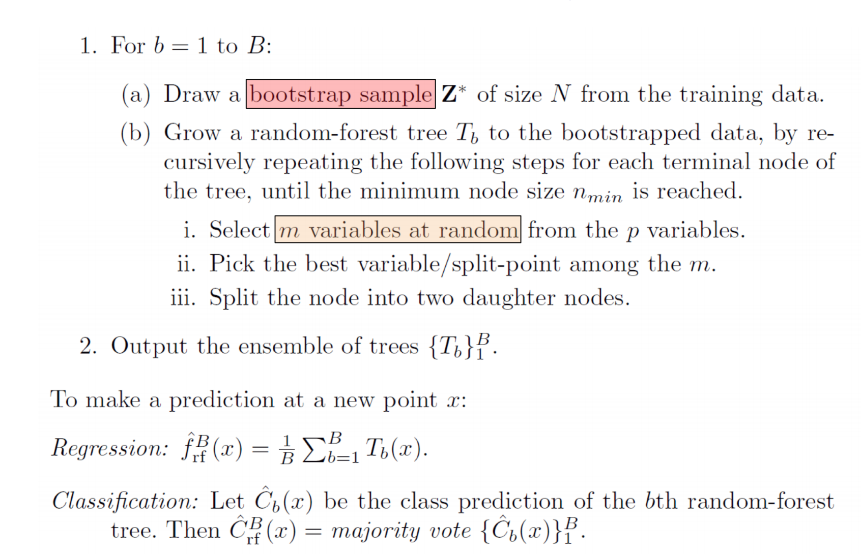
Note that in Random Forest algorithm, each time you make a tree, you make a full sized tree. Some trees might be bigger than others bu there is no predetermined maximum depth.

Predictions in Random Forest

When it comes time to make a prediction, the random forest takes plain average of all the individual decision tree estimates in the case for a regression task. For classification, the random forest will take a majority vote for the predicted class.

Advantages and Disadvantages of Random Forest

The procedure is easy to implement: only two parameters are to be set (number of trees and the number of variables considered at each split). We follow the recommendations of Breiman, 2001 and use a large number of trees (1000) and the sqrt(p) as the size of the variable subsets where p is the total number of variables. We can also choose the number of variables to be selected at each split using Cross-Validation.

Random forests does not overfit. You can run as many trees as you want. It is fast.

It is versatile. It can handle binary features, categorical features, and numerical features. There is very little pre-processing that needs to be done.

Random Forest handles higher dimensionality data very well. Instead of using all the features of your problem, individual trees only use a subset of the features. This minimizes the space that each tree is optimizing over and can help combat the problem of the curse of dimensionality.

Random forests has two ways of replacing missing values. The first way is fast and uni-variate approach (treat each variable as independent). If the $m$th variable is not categorical, the method computes the median of all values of this variable in class $j$, then it uses this value to replace all missing values of the $m$th variable in class $j$. If the $m$th variable is categorical, the replacement is the most frequent non-missing value in class $j$. These replacement values are called fills.

After each tree is built, all of the data are run down the tree, and proximities are computed for each pair of cases. The proximities originally formed a $N \times N$ matrix. If two cases occupy the same terminal node, their proximity is increased by one. At the end of the run, the proximities are normalized by dividing by the number of trees. Proximities are used in replacing missing data, locating outliers, and producing illuminating low-dimensional views of the data.

It replaces missing values only in the training set. It begins by doing a rough and inaccurate filling in of the missing values. Then it does a forest run and computes proximities. If $x(m,n)$ is a missing continuous value, estimate its fill as an average over the non-missing values of the $m$th variables weighted by the proximities between the $n$th case and the non-missing value case. If it is a missing categorical variable, replace it by the most frequent non-missing value where frequency is weighted by proximity. Now iterate-construct a forest again using these newly filled in values, find new fills and iterate again. Our experience is that 4-6 iterations are enough.

Missing value replacement for the test set is a little different. When there is a test set, there are two different methods of replacement depending on whether labels exist for the test set. If label (class information) for this test case exists, then the fills derived from the training set are used as replacements. If labels do not exist, then each case in the test set is replicated nclass times (nclass= number of classes). The first replicate of a case is assumed to be class 1 and the class one fills used to replace missing values. The 2nd replicate is assumed class 2 and the class 2 fills used on it. This augmented test set is run down the tree. In each set of replicates, the one receiving the most votes determines the class of the original case.

On online materials, you can see that Random Forest is usually robust to outliers. However, that is not the whole story. It is not the Random Forest algorithm itself that is robust to outliers, but the base learner it is based on: the decision tree. Decision trees isolate atypical observations into small leaves (i.e., small subspaces of the original space). Furthermore, decision trees are local models. Unlike linear regression, where the same equation holds for the entire space, a very simple model is fitted locally to each subspace (i.e., to each leaf). In the case of regression, it is generally a very low-order regression model (usually only the average of the observations in the leaf). For classification, it is majority voting. Therefore, for regression for instance, extreme values do not affect the entire model because they get averaged locally. So the fit to the other values is not affected. So, in a nutshell, RF inherits its insensitivity to outliers from recursive partitioning and local model fitting.

Random Forest uses bootstrap sampling and feature sampling, i.e row sampling and column sampling. Therefore Random Forest is not affected by multicollinearity that much since it is picking different set of features for different models and of course every model sees a different set of data points. But there is a chance of multicollinear features getting picked up together, and when that happens we will see some trace of it. Feature importance will definitely be affected by multicollinearity. Intuitively, if the features have same effect or there is a relation in between the features, it can be difficult to rank the relative importance of features. In other words, it’s not easy to say which one is even if we can access the underlying effect by measuring more than one variable, or if they are mutual symptoms of a third effect.

No feature scaling (standardization and normalization) required in case of Random Forest as it uses rule based approach instead of distance calculation.

It is parallelizable: You can distribute the computations across multiple processors and build all the trees in parallel.

Similar to other ensemble methods, interprebility is a problem for Random Forests algorithm too.

It’s more complex and computationally expensive than decision tree algorithm, which makes the algorithm slow and ineffective for real-time predictions, due to a large number of trees, as a more accurate prediction requires more trees.

It cannot extrapolate at all to data that are outside the range that they have seen. The reason is simple: the predictions from a Random Forest are done through averaging the results obtained in several trees. The trees themselves output the mean value of the samples in each terminal node, the leaves. It’s impossible for the result to be outside the range of the training data, because the average is always inside the range of its constituents. In other words, it’s impossible for an average to be bigger (or lower) than every sample, and Random Forests regressions are based on averaging.

OOB Evaluation in Random Forest

The out of bag samples associated with each tree in a RandomForestClassifier will be different from one tree to another. Each of the OOB sample rows is passed through every Decision Trees that did not contain the OOB sample row in its bootstrap training data and a majority prediction is noted for each row.

For more: https://towardsdatascience.com/what-is-out-of-bag-oob-score-in-random-forest-a7fa23d710

import numpy as np
import pandas as pd
import matplotlib.pyplot as plt
%matplotlib inline
from sklearn.metrics import accuracy_score
from sklearn.model_selection import train_test_split
from sklearn.datasets import make_moons
from sklearn.ensemble import RandomForestClassifier
from sklearn.tree import export_graphviz
import pydot

X, y = make_moons(n_samples=1000, noise=0.30, random_state=42)
X_train, X_test, y_train, y_test = train_test_split(X, y, random_state=42)

rnd_clf = RandomForestClassifier(n_estimators=10, oob_score = True, random_state=42)
rnd_clf.fit(X_train, y_train)

y_pred_rf = rnd_clf.predict(X_test)

print('Accuracy of Random Forest algorithm: {}'.format(accuracy_score(y_test, y_pred_rf)))
#Accuracy of Random Forest algorithm: 0.872

print('OOB score is {}'.format(rnd_clf.oob_score_))
#OOB score is 0.8893333333333333


#The command below gives all the trees built in the forest
rnd_clf.estimators_
# [DecisionTreeClassifier(class_weight=None, criterion='gini', max_depth=None,
#              max_features='auto', max_leaf_nodes=None,
#              min_impurity_decrease=0.0, min_impurity_split=None,
#              min_samples_leaf=1, min_samples_split=2,
#              min_weight_fraction_leaf=0.0, presort=False,
#              random_state=1608637542, splitter='best'),
#  DecisionTreeClassifier(class_weight=None, criterion='gini', max_depth=None,
#              max_features='auto', max_leaf_nodes=None,
#              min_impurity_decrease=0.0, min_impurity_split=None,
#              min_samples_leaf=1, min_samples_split=2,
#              min_weight_fraction_leaf=0.0, presort=False,
#              random_state=1273642419, splitter='best'),
#  DecisionTreeClassifier(class_weight=None, criterion='gini', max_depth=None,
#              max_features='auto', max_leaf_nodes=None,
#              min_impurity_decrease=0.0, min_impurity_split=None,
#              min_samples_leaf=1, min_samples_split=2,
#              min_weight_fraction_leaf=0.0, presort=False,
#              random_state=1935803228, splitter='best'),
#  DecisionTreeClassifier(class_weight=None, criterion='gini', max_depth=None,
#              max_features='auto', max_leaf_nodes=None,
#              min_impurity_decrease=0.0, min_impurity_split=None,
#              min_samples_leaf=1, min_samples_split=2,
#              min_weight_fraction_leaf=0.0, presort=False,
#              random_state=787846414, splitter='best'),
#  DecisionTreeClassifier(class_weight=None, criterion='gini', max_depth=None,
#              max_features='auto', max_leaf_nodes=None,
#              min_impurity_decrease=0.0, min_impurity_split=None,
#              min_samples_leaf=1, min_samples_split=2,
#              min_weight_fraction_leaf=0.0, presort=False,
#              random_state=996406378, splitter='best'),
#  DecisionTreeClassifier(class_weight=None, criterion='gini', max_depth=None,
#              max_features='auto', max_leaf_nodes=None,
#              min_impurity_decrease=0.0, min_impurity_split=None,
#              min_samples_leaf=1, min_samples_split=2,
#              min_weight_fraction_leaf=0.0, presort=False,
#              random_state=1201263687, splitter='best'),
#  DecisionTreeClassifier(class_weight=None, criterion='gini', max_depth=None,
#              max_features='auto', max_leaf_nodes=None,
#              min_impurity_decrease=0.0, min_impurity_split=None,
#              min_samples_leaf=1, min_samples_split=2,
#              min_weight_fraction_leaf=0.0, presort=False,
#              random_state=423734972, splitter='best'),
#  DecisionTreeClassifier(class_weight=None, criterion='gini', max_depth=None,
#              max_features='auto', max_leaf_nodes=None,
#              min_impurity_decrease=0.0, min_impurity_split=None,
#              min_samples_leaf=1, min_samples_split=2,
#              min_weight_fraction_leaf=0.0, presort=False,
#              random_state=415968276, splitter='best'),
#  DecisionTreeClassifier(class_weight=None, criterion='gini', max_depth=None,
#              max_features='auto', max_leaf_nodes=None,
#              min_impurity_decrease=0.0, min_impurity_split=None,
#              min_samples_leaf=1, min_samples_split=2,
#              min_weight_fraction_leaf=0.0, presort=False,
#              random_state=670094950, splitter='best'),
#  DecisionTreeClassifier(class_weight=None, criterion='gini', max_depth=None,
#              max_features='auto', max_leaf_nodes=None,
#              min_impurity_decrease=0.0, min_impurity_split=None,
#              min_samples_leaf=1, min_samples_split=2,
#              min_weight_fraction_leaf=0.0, presort=False,
#              random_state=1914837113, splitter='best')]

# Extract the fifth tree
fifth_small = rnd_clf.estimators_[5]

# Save the tree as a png image
export_graphviz(fifth_small, out_file = 'fifth_tree.dot', feature_names = ['Feature 1', 'Feature 2'], class_names=['0','1'], rounded = True, precision = 1)
(graph, ) = pydot.graph_from_dot_file('fifth_tree.dot')
graph.write_png('fifth_tree.png');

The tree we will have from the command above will be enourmous since we have not defined max_depth in RandomForestClassifier. It is None. If None, then nodes are expanded until all leaves are pure or until all leaves contain less than min_samples_split samples.

Feature Importance

Yet another great quality of Random Forests is that they make it easy to measure the relative importance of each feature. Scikit-Learn computes this score automatically for each feature after training. You can access the result using the feature_importances_ variable.

# Load libraries
from sklearn.ensemble import RandomForestClassifier
from sklearn import datasets
import numpy as np
import matplotlib.pyplot as plt

# Load data
iris = datasets.load_iris()
X = iris.data
y = iris.target

# Create decision tree classifer object
clf = RandomForestClassifier(n_estimators=500, max_leaf_nodes = 16, random_state=0, n_jobs=-1)

# Train model
model = clf.fit(X, y)

#If you have a test set, you can evaluate the algorithm as the following:
# y_pred_rf = rnd_clf.predict(X_test)
# from sklearn.metrics import accuracy_score
# print('Accuracy of Random Forest algorithm: {}'.format(accuracy_score(y_test, y_pred_rf)))

# Calculate feature importances
importances = model.feature_importances_
#array([0.09539456, 0.02274582, 0.44094962, 0.44090999])

# Sort feature importances in descending order
indices = np.argsort(importances)[::-1]

# Rearrange feature names so they match the sorted feature importances
names = [iris.feature_names[i] for i in indices]

# Create plot
plt.figure()

# Create plot title
plt.title("Feature Importance")

# Add bars
plt.bar(range(X.shape[1]), importances[indices])

# Add feature names as x-axis labels
plt.xticks(range(X.shape[1]), names, rotation=90)

# Show plot
plt.show()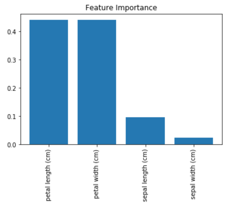

BOOSTING

Originally called hypothesis boosting, boosting refers to any Ensemble method that can combine several “weak” learners with low variance but high bias (The weak learners in AdaBoost are decision trees with a single split, called decision stumps (1-level decision trees)) into a strong learner with a lower bias than its components. A weak learner is a constrained model (i.e. you could limit the max depth of each decision tree). Those weak learners are very basic classifiers doing only slightly better than a random guess.

The general idea of most boosting methods is that new models are added to correct the errors made by existing models. Models are added sequentially until no further improvements can be made (each trying to correct its predecessor).

Boosting can be used primarily for reducing bias, that is, models that underfit the training data. However, they can still overfit due to the number of iteration; therefore, the iteration process should be stopped to avoid it. To combat overfitting is usually as simple as using cross validation to determine how many boosting steps to take.

The basic motivation of sequential methods is to exploit the dependence between the base learners. The overall performance can be boosted by weighing previously mislabeled examples with higher weight.

There are many boosting algorithms available but here we will focus on Adaptive Boosting (AdaBoost) and Gradient Boosting.

Adaptive Boosting

AdaBoost was the first really successful boosting algorithm developed for binary classification. In AdaBoost, classifiers are trained on weighted versions of the dataset, and then combined to produce a final prediction.

One way for a new predictor to correct its predecessor is to pay a bit more attention to the training instances that the predecessor underfitted. This results in new predictors focusing more and more on the hard cases. For example, to build an AdaBoost classifier, it begins by training a decision tree in which each observation is assigned an equal weight. A first base classifier (such as a Decision Tree) is trained and used to make predictions on the training set. The observation weights are individually modified and the weight of misclassified training instances is then increased. A second classifier is then reapplied to the weighted observations and again it makes predictions on the training set, weights are updated, and so on. The first classifier gets many instances wrong, so their weights get boosted. The second classifier therefore does a better job on these instances, and so on. Once all predictors are trained, the ensemble makes predictions very much like bagging or pasting, except that predictors have different weights depending on their overall accuracy on the weighted training set. There is one important drawback to this sequential learning technique: it cannot be parallelized (or only partially), since each predictor can only be trained after the previous predictor has been trained and evaluated. As a result, it does not scale as well as bagging or pasting.

We begin by describing the algorithm itself. Consider a two-class problem, with the output variable coded as $Y \in \{−1, 1\}$. Given a vector of predictor variables $X$, a classifier $G(X)$ produces a prediction taking one of the two values ${−1, 1}$. The error rate on the training sample is:

A weak classifier is one whose error rate is only slightly better than random guessing. The purpose of boosting is to sequentially apply the weak classification algorithm to repeatedly modified versions of the data, thereby producing a sequence of weak classifiers $G_{m}(x), m = 1, 2, \cdots , M$. The algorithm belows shows the steps:

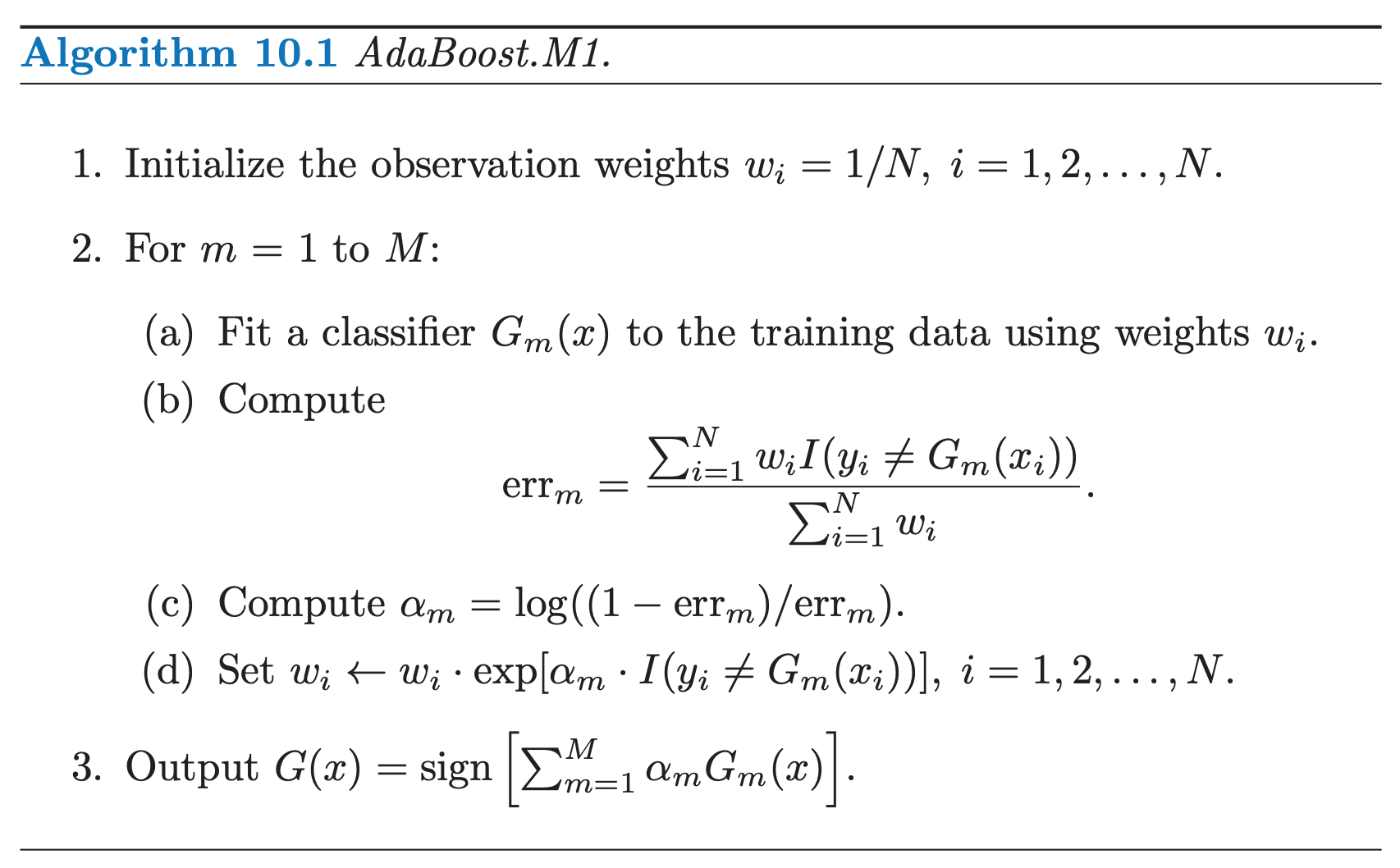
Here, $I(\cdot)$ is the indicator function, where $I(y_{i} \neq G_{m}(x_{i})) = 1$ if $G_{m}(x_{i}) \neq y_{i}$ and 0 otherwise.

As can be seen from Step 2.d, observations misclassified by $G_{m}(x)$ have their weights scaled by a factor $exp(\alpha_{m})$, increasing their relative influence for inducing the next classifier $G_{m+1}(x)$ in the sequence.

NOTE that sometimes, in order avoid numerical instability, after step 2d, we can normalize the weights at each step, $w_i \leftarrow \frac{w_i}{\sum_{i=1}^N w_i}$

The original implementation does not use a learning rate parameter. In some implementation, at the step 2c, we multiply estimator weight ($\alpha_{m}$) with a learning rate, i.e. $\alpha_m = \text{learning_rate} \times \log \left( \frac{1 - err_m}{err_m}\right)$. It is a scalar value which shrinks the contribution of each classifier by $\text{learning_rate}$ and slows down the learning. It is used to make smaller steps to practically avoid overfitting our data. This parameter controls how much we are going to contribute with the new model to the existing one. Normally there is trade off between the number of iterations (every iteration AdaBoost algorithm trains a new classifier, $i = 1, 2, \dots , M$. Hence number of classifiers equals number of iterations) and the value of learning rate. In other words, when taking smaller values of learning rate, you should consider more $M$ iterations (the model needs longer to train), so that your base model (the weak classifier) continues to improve. According to Jerome Friedman, it is suggested to set learning to smaller values , such as less than $0.1$.

The algorithm defined above is known as “Discrete AdaBoost” because the base classifier $G_{m}(x)$ returns a discrete class label. If the base classifier instead returns a real-valued prediction (e.g., a probability mapped to the interval $[−1, 1]$), AdaBoost can be modified appropriately.

Scikit-Learn actually uses a multiclass version of AdaBoost called SAMME (which stands for Stagewise Additive Modeling using a Multiclass Exponential loss function). When there are just two classes, SAMME is equivalent to AdaBoost.

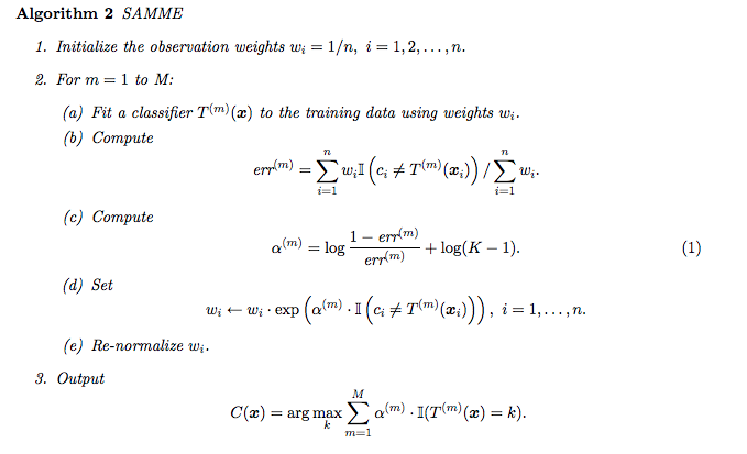
Moreover, if the predictors can estimate class probabilities (i.e., if they have a predict_proba() method), Scikit-Learn can use a variant of SAMME called SAMME.R (the R stands for “Real”), which relies on class probabilities rather than predictions and generally performs better.

The number of iterations needed for AdaBoost depends on the problem. Mease and Wyner (2008) argue that AdaBoost should be run for a long time, until it converges, and that 1,000 iterations should be enough.

AdaBoost suffer from the curse of dimensionality which can lead to overfitting. However, it certainly does not explicitly regularize — there is nothing about the algorithm that overtly limits the weights on the weak hypotheses. But, it avoids overfitting through implicit regularization. One thing in mind is that the iteration process should be stopped to avoid it. If your AdaBoost ensemble is overfitting the training set, you can try reducing the number of estimators or more strongly regularizing the base estimator (for example, decision trees in this case). If it underfits the training data, you can try increasing the number of base estimators or reducing the regularization hyperparameters of the base estimator.

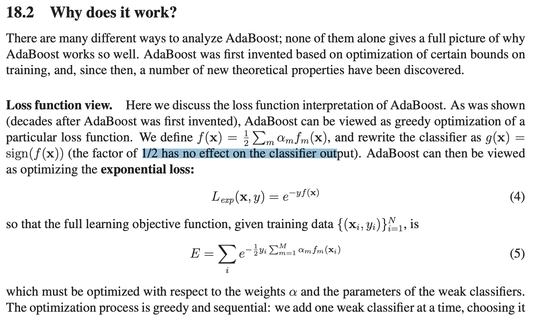
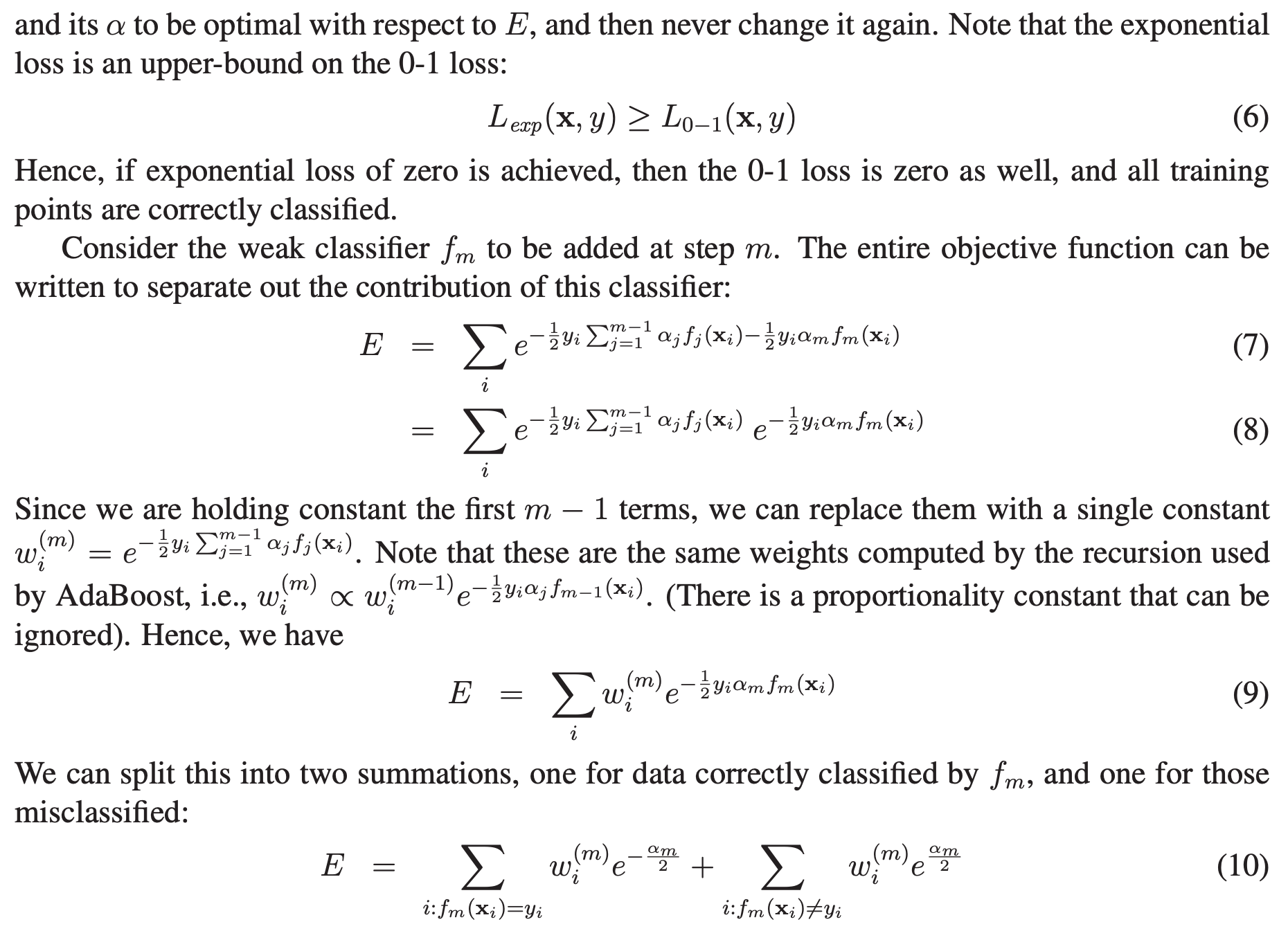
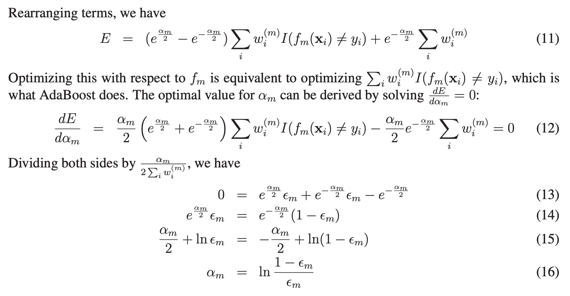
NOTE : Many, perhaps even most, learning and statistical methods, that are in common use, can be viewed as procedures for minimizing a loss function (also called a cost or objective function) that in some way measures how well a model fits the observed data. A classic example is least-squares regression in which a sum of squared errors is minimized. Though not originally designed for this purpose, it was later discovered that AdaBoost can also be expressed as in terms of the more general framework of additive models with a particular loss function (the exponential loss) to be minimized.

Viewing the algorithm in this light can be helpful for a number of reasons. First, such an understanding can help to clarify the goal of the algorithm and can be useful in proving convergence properties. And second, by decoupling the algorithm from its objective, we may be able to derive better or faster algorithms for the same objective, or alternatively, we might be able to generalize AdaBoost for new challenges.

Details can be seen here here.

Predictions with AdaBoost

Predictions are made by calculating the weighted average of the weak classifiers.

For a new input instance, each weak learner calculates a predicted value as either +1.0 or -1.0. The predicted values are weighted by each weak learners stage value. The prediction for the ensemble model is taken as a the sum of the weighted predictions. If the sum is positive, then the first class is predicted, if it is negative, the second class is predicted.

where $M$ the number of models (i.e., ensemble size) and $G_{m}(x) \in [-1,1]$ and $\alpha_{m}$’s are stage values for the model $m$. Note that at the first step $m = 1$ the weights are initialized uniformly $w_{i} = 1/N$ where $N$ is the sample size.

For example, 5 weak classifiers may predict the values 1.0, 1.0, -1.0, 1.0, -1.0. From a majority vote, it looks like the model will predict a value of 1.0 or the first class. These same 5 weak classifiers may have the stage values 0.2, 0.5, 0.8, 0.2 and 0.9 respectively. Calculating the weighted sum of these predictions results in an output of -0.8, which would be an ensemble prediction of -1.0 or the second class.

# Load libraries
from sklearn.ensemble import AdaBoostClassifier
from sklearn.tree import DecisionTreeClassifier
from sklearn import datasets
# Import train_test_split function
from sklearn.model_selection import train_test_split
from sklearn.metrics import accuracy_score

# Load data
iris = datasets.load_iris()
X = iris.data
y = iris.target

# Split dataset into training set and test set
X_train, X_test, y_train, y_test = train_test_split(X, y, test_size=0.3) # 70% training and 30% test

#The base estimator from which the boosted ensemble is built. AdaBoost uses Decision Tree Classifier as default Classifier.
#One can use different base estimator. 

#If ‘SAMME.R’ then use the SAMME.R real boosting algorithm. base_estimator must support calculation of class probabilities. 
#If ‘SAMME’ then use the SAMME discrete boosting algorithm. The SAMME.R algorithm typically converges faster than SAMME, 
#achieving a lower test error with fewer boosting iterations.
ada_clf = AdaBoostClassifier(
    DecisionTreeClassifier(max_depth=1), n_estimators=200,
    algorithm="SAMME.R", learning_rate=0.5, random_state=42)
ada_clf.fit(X_train, y_train)

# Train Adaboost Classifer
ada_clf.fit(X_train, y_train)

#Predict the response for test dataset
y_pred_AdaBoost = ada_clf.predict(X_test)

print('Accuracy of AdaBoost algorithm: {}'.format(accuracy_score(y_test, y_pred_AdaBoost)))
#Accuracy of AdaBoost algorithm: 0.9111111111111111

Implementation from scratch

import numpy as np
from sklearn.tree import DecisionTreeClassifier
from sklearn.ensemble import AdaBoostClassifier

#Toy Dataset
x1 = np.array([.1,.2,.4,.8, .8, .05,.08,.12,.33,.55,.66,.77,.88,.2,.3,.4,.5,.6,.25,.3,.5,.7,.6])
x2 = np.array([.2,.65,.7,.6, .3,.1,.4,.66,.77,.65,.68,.55,.44,.1,.3,.4,.3,.15,.15,.5,.55,.2,.4])
y = np.array([1,1,1,1,1,1,1,1,1,1,1,1,1,-1,-1,-1,-1,-1,-1,-1,-1,-1,-1])
X = np.vstack((x1,x2)).T

# Using Scikit-Learn
classifier = AdaBoostClassifier(base_estimator = DecisionTreeClassifier(max_depth = 1, max_leaf_nodes=2), algorithm = 'SAMME', n_estimators=10, learning_rate=1.0)
classifier.fit(X, y)
print(f'Accuracy from Scikit Learn function = {classifier.score(X,y)}')

# From scratch 

M = 10 # number of estimators
learning_rate = 1.0
N = len(y) #number of samples in the dataset

sample_weight_list = []
estimator_list = []
y_predict_list = []
estimator_error_list = []
estimator_weight_list = []

#Initialize the sample weights
sample_weight = np.ones(N) / N # first weights assigned uniformly to data points
sample_weight_list.append(sample_weight.copy())

#For m = 1 to M
for m in range(M):
    #Fit a classifier
    #AdaBoost almost always a decision stump
    estimator = DecisionTreeClassifier(max_depth = 1, max_leaf_nodes=2)
    estimator.fit(X, y, sample_weight=sample_weight)
    y_predict = estimator.predict(X)
    
    #Misclassifications
    incorrect = (y_predict != y)

    #Estimator error
    estimator_error = np.mean( np.average(incorrect, weights=sample_weight, axis=0))
    
    #Boost estimator weights
    estimator_weight =  learning_rate * np.log((1. - estimator_error) / estimator_error)
    
    #Boost sample weights
    sample_weight *= np.exp(estimator_weight * incorrect * ((sample_weight > 0) | (estimator_weight < 0)))
    
    #Save iteration values
    estimator_list.append(estimator)
    y_predict_list.append(y_predict.copy())
    estimator_error_list.append(estimator_error.copy())
    estimator_weight_list.append(estimator_weight.copy())
    sample_weight_list.append(sample_weight.copy())
    
#Convert to np array for convenience   
estimator_list = np.asarray(estimator_list)
y_predict_list = np.asarray(y_predict_list)
estimator_error_list = np.asarray(estimator_error_list)
estimator_weight_list = np.asarray(estimator_weight_list)
sample_weight_list = np.asarray(sample_weight_list)

#Predictions
preds = (np.array([np.sign((y_predict_list[:,point] * estimator_weight_list).sum()) for point in range(N)]))
print('Accuracy from the implementation from scratch = ', (preds == y).sum() / N)

Gradient Boosting

Another very popular Boosting algorithm is Gradient Boosting. It gets its name from the combination of Gradient Descent algorithm and Boosting.

Just like AdaBoost, Gradient Boosting adds predictors to an ensemble in a gradual, additive and sequential manner, each one correcting its predecessor. However, instead of tweaking the instance weights at every iteration like AdaBoost does, this method tries to fit the new predictor to the residual errors made by the previous predictor because errors of early predictions indicate the “hard” examples. Like AdaBoost, gradient boosting scales the trees but unlike AdaBoost, it scales all trees by the same amount.

Let’s go through a simple regression example using Decision Trees as the base predictors (of course Gradient Boosting works great with regression tasks) This is called Gradient Tree Boosting or Gradient Boosted Regression Trees (GBRT). First let’s fit DecisionTreeRegressor to the training set (for example, a noist quadratic training set):

#Let's create some data
import numpy as np
np.random.seed(42)
X = np.random.rand(100, 1) - 0.5
y = 3*X[:, 0]**2 + 0.05 * np.random.randn(100)

from sklearn.tree import DecisionTreeRegressor

tree_reg1 = DecisionTreeRegressor(max_depth=2, random_state=42)
tree_reg1.fit(X, y)
# DecisionTreeRegressor(criterion='mse', max_depth=2, max_features=None,
#            max_leaf_nodes=None, min_impurity_decrease=0.0,
#            min_impurity_split=None, min_samples_leaf=1,
#            min_samples_split=2, min_weight_fraction_leaf=0.0,
#            presort=False, random_state=42, splitter='best')

Now train a second DecisionTreeRegressor on the residual errors made by the first predictor:

y2 = y - tree_reg1.predict(X)
tree_reg2 = DecisionTreeRegressor(max_depth=2, random_state=42)
tree_reg2.fit(X, y2)
# DecisionTreeRegressor(criterion='mse', max_depth=2, max_features=None,
#            max_leaf_nodes=None, min_impurity_decrease=0.0,
#            min_impurity_split=None, min_samples_leaf=1,
#            min_samples_split=2, min_weight_fraction_leaf=0.0,
#            presort=False, random_state=42, splitter='best')

Then we train a third regressor on the residual errors made by the second predictor

y3 = y2 - tree_reg2.predict(X)
tree_reg3 = DecisionTreeRegressor(max_depth=2, random_state=42)
tree_reg3.fit(X, y3)
# DecisionTreeRegressor(criterion='mse', max_depth=2, max_features=None,
#            max_leaf_nodes=None, min_impurity_decrease=0.0,
#            min_impurity_split=None, min_samples_leaf=1,
#            min_samples_split=2, min_weight_fraction_leaf=0.0,
#            presort=False, random_state=42, splitter='best')

Now we have an ensemble containing three trees. It can make predictions on a new instance simply by adding up the predictions of all the trees:

X_new = np.array([[0.8]])
y_pred = sum(tree.predict(X_new) for tree in (tree_reg1, tree_reg2, tree_reg3))
print(y_pred)
#[0.75026781]

import matplotlib.pyplot as plt

def plot_predictions(regressors, X, y, axes, label=None, style="r-", data_style="b.", data_label=None):
    x1 = np.linspace(axes[0], axes[1], 500)
    y_pred = sum(regressor.predict(x1.reshape(-1, 1)) for regressor in regressors)
    plt.plot(X[:, 0], y, data_style, label=data_label)
    plt.plot(x1, y_pred, style, linewidth=2, label=label)
    if label or data_label:
        plt.legend(loc="upper center", fontsize=16)
    plt.axis(axes)

plt.figure(figsize=(11,11))

plt.subplot(321)
plot_predictions([tree_reg1], X, y, axes=[-0.5, 0.5, -0.1, 0.8], label="$h_1(x_1)$", style="g-", data_label="Training set")
plt.ylabel("$y$", fontsize=16, rotation=0)
plt.title("Residuals and tree predictions", fontsize=16)

plt.subplot(322)
plot_predictions([tree_reg1], X, y, axes=[-0.5, 0.5, -0.1, 0.8], label="$h(x_1) = h_1(x_1)$", data_label="Training set")
plt.ylabel("$y$", fontsize=16, rotation=0)
plt.title("Ensemble predictions", fontsize=16)

plt.subplot(323)
plot_predictions([tree_reg2], X, y2, axes=[-0.5, 0.5, -0.5, 0.5], label="$h_2(x_1)$", style="g-", data_style="k+", data_label="Residuals")
plt.ylabel("$y - h_1(x_1)$", fontsize=16)

plt.subplot(324)
plot_predictions([tree_reg1, tree_reg2], X, y, axes=[-0.5, 0.5, -0.1, 0.8], label="$h(x_1) = h_1(x_1) + h_2(x_1)$")
plt.ylabel("$y$", fontsize=16, rotation=0)

plt.subplot(325)
plot_predictions([tree_reg3], X, y3, axes=[-0.5, 0.5, -0.5, 0.5], label="$h_3(x_1)$", style="g-", data_style="k+")
plt.ylabel("$y - h_1(x_1) - h_2(x_1)$", fontsize=16)
plt.xlabel("$x_1$", fontsize=16)

plt.subplot(326)
plot_predictions([tree_reg1, tree_reg2, tree_reg3], X, y, axes=[-0.5, 0.5, -0.1, 0.8], label="$h(x_1) = h_1(x_1) + h_2(x_1) + h_3(x_1)$")
plt.xlabel("$x_1$", fontsize=16)
plt.ylabel("$y$", fontsize=16, rotation=0)

plt.show()

Plots represents the predictions of these three trees in the left column, and the ensemble’s predictions in the right column. In the first row, the ensemble has just one tree, so its predictions are exactly the same as the first tree’s predictions. In the second row, a new tree is trained on the residual errors of the first tree. On the right you can see that the ensemble’s predictions are equal to the sum of the predictions of the first two trees. Similarly, in the third row another tree is trained on the residual errors of the second tree. You can see that the ensemble’s predictions gradually get better as trees are added to the ensemble.

A simpler way to train GBRT ensembles is to use Scikit-Learn’s GradientBoostingRegressor class. Much like the RandomForestRegressor class, it has hyperparameters to control the growth of Decision Trees (e.g., max_depth, min_samples_leaf, and so on), as well as hyperparameters to control the ensemble training, such as the number of trees (n_estimators). The following code creates the same ensemble as the previous one:

from sklearn.ensemble import GradientBoostingRegressor
gbrt = GradientBoostingRegressor(max_depth=2, n_estimators=3, learning_rate=1.0)
gbrt.fit(X, y)

X_new = np.array([[0.8]])
y_pred = gbrt.predict(X_new)
print(y_pred)
#[0.75026781]

The three principal hyperparameters to tune in gradient boosting are the number of the trees, the learning rate and the dept of trees - all three affect the model performance, The dept of the tree also affects the speed of training and prediction: the shorter, the faster.

The learning_rate hyperparameter scales the contribution of each tree. It essentially slows down the learning. If you set it to a low value, such as 0.1, you will need more trees in the ensemble to fit the training set, but the predictions will usually generalize better. This is a regularization technique called shrinkage. If your Gradient Boosting ensemble overfits the training data, you should try to decrease the learning rate. You could also use early stopping to find the right number of predictors (you probably have too many).

from sklearn.ensemble import GradientBoostingRegressor
import matplotlib.pyplot as plt
import numpy as np

def plot_predictions(regressors, X, y, axes, label=None, style="r-", data_style="b.", data_label=None):
    x1 = np.linspace(axes[0], axes[1], 500)
    y_pred = sum(regressor.predict(x1.reshape(-1, 1)) for regressor in regressors)
    plt.plot(X[:, 0], y, data_style, label=data_label)
    plt.plot(x1, y_pred, style, linewidth=2, label=label)
    if label or data_label:
        plt.legend(loc="upper center", fontsize=16)
    plt.axis(axes)
    
    
np.random.seed(42)
X = np.random.rand(100, 1) - 0.5
y = 3*X[:, 0]**2 + 0.05 * np.random.randn(100)

gbrt = GradientBoostingRegressor(max_depth=2, n_estimators=3, learning_rate=1.0, random_state=42)
gbrt.fit(X, y)

gbrt_slow = GradientBoostingRegressor(max_depth=2, n_estimators=200, learning_rate=0.1, random_state=42)
gbrt_slow.fit(X, y)

plt.figure(figsize=(11,4))

plt.subplot(121)
plot_predictions([gbrt], X, y, axes=[-0.5, 0.5, -0.1, 0.8], label="Ensemble predictions")
plt.title("learning_rate={}, n_estimators={}".format(gbrt.learning_rate, gbrt.n_estimators), fontsize=14)

plt.subplot(122)
plot_predictions([gbrt_slow], X, y, axes=[-0.5, 0.5, -0.1, 0.8])
plt.title("learning_rate={}, n_estimators={}".format(gbrt_slow.learning_rate, gbrt_slow.n_estimators), fontsize=14)

plt.show()

Figure shows two GBRT ensembles trained with a low learning rate: the one on the left does not have enough trees to fit the training set, while the one on the right has too many trees and overfits the training set. (decreasing the learning rate might help).

In order to find the optimal number of trees, you can use early stopping. A simple way to implement this is to use the staged_predict() method: it returns an iterator over the predictions made by the ensemble at each stage of training (with one tree, two trees, etc.). The following code trains a GBRT ensemble with 120 trees, then measures the validation error at each stage of training to find the optimal number of trees, and finally trains another GBRT ensemble using the optimal number of trees:

import numpy as np
from sklearn.model_selection import train_test_split
from sklearn.metrics import mean_squared_error
from sklearn.ensemble import GradientBoostingRegressor

np.random.seed(42)
X = np.random.rand(100, 1) - 0.5
y = 3*X[:, 0]**2 + 0.05 * np.random.randn(100)

X_train, X_val, y_train, y_val = train_test_split(X, y, random_state=49)

gbrt = GradientBoostingRegressor(max_depth=2, n_estimators=120, random_state=42)
gbrt.fit(X_train, y_train)

errors = [mean_squared_error(y_val, y_pred)
          for y_pred in gbrt.staged_predict(X_val)]

#len(errors) = 120 because we are trying models with number of trees up to 120

bst_n_estimators = np.argmin(errors) + 1

gbrt_best = GradientBoostingRegressor(max_depth=2,n_estimators=bst_n_estimators, random_state=42)
gbrt_best.fit(X_train, y_train)

min_error = np.min(errors)
#0.002712853325235463

import matplotlib.pyplot as plt

def plot_predictions(regressors, X, y, axes, label=None, style="r-", data_style="b.", data_label=None):
    x1 = np.linspace(axes[0], axes[1], 500)
    y_pred = sum(regressor.predict(x1.reshape(-1, 1)) for regressor in regressors)
    plt.plot(X[:, 0], y, data_style, label=data_label)
    plt.plot(x1, y_pred, style, linewidth=2, label=label)
    if label or data_label:
        plt.legend(loc="upper center", fontsize=16)
    plt.axis(axes)
plt.figure(figsize=(11, 4))
plt.subplot(121)
plt.plot(errors, "b.-")
plt.plot([bst_n_estimators, bst_n_estimators], [0, min_error], "k--")
plt.plot([0, 120], [min_error, min_error], "k--")
plt.plot(bst_n_estimators, min_error, "ko")
plt.text(bst_n_estimators, min_error*1.2, "Minimum", ha="center", fontsize=14)
plt.axis([0, 120, 0, 0.01])
plt.xlabel("Number of trees")
plt.title("Validation error", fontsize=14)

plt.subplot(122)
plot_predictions([gbrt_best], X, y, axes=[-0.5, 0.5, -0.1, 0.8])
plt.title("Best model (%d trees)" % bst_n_estimators, fontsize=14)

plt.show()

It is also possible to implement early stopping by actually stopping training early (instead of training a large number of trees first and then looking back to find the optimal number). You can do so by setting warm_start=True, which makes Scikit- Learn keep existing trees when the fit() method is called, allowing incremental training. The following code stops training when the validation error does not improve for five iterations in a row:

import numpy as np
from sklearn.model_selection import train_test_split
from sklearn.ensemble import GradientBoostingRegressor

np.random.seed(42)
X = np.random.rand(100, 1) - 0.5
y = 3*X[:, 0]**2 + 0.05 * np.random.randn(100)

X_train, X_val, y_train, y_val = train_test_split(X, y, random_state=49)

gbrt = GradientBoostingRegressor(max_depth=2, warm_start=True, random_state=42)

#There is no difference between np.inf and float("inf") and they can be used interchangeably.
min_val_error = np.inf
error_going_up = 0
for n_estimators in range(1, 120):
    gbrt.n_estimators = n_estimators
    gbrt.fit(X_train, y_train)
    y_pred = gbrt.predict(X_val)
    val_error = mean_squared_error(y_val, y_pred)
    if val_error < min_val_error:
        min_val_error = val_error
        error_going_up = 0
    else:
        error_going_up += 1
        if error_going_up == 5:
            break  # early stopping
            
print(gbrt.n_estimators)
#61

print("Minimum validation MSE:", min_val_error)
#Minimum validation MSE: 0.002712853325235463

Boosting reduces the bias (or underfitting) instead of variance. Thus, boosting can overfit. However, by tuning the hyperparameters, overfitting can be largely avoided. It usually outperforms random forest in accuracy but because of its sequential nature, can be significantly slower in training.

XGBoost

XGBoost stands for eXtreme Gradient Boosting. XGBoost is an implementation of gradient boosted decision trees designed for speed and performance. Gradient boosting machines are generally very slow in implementation because of sequential model training. Hence, they are not very scalable. Thus, XGBoost is focused on computational speed and model performance. XGBoost provides:

• Parallelization of tree construction using all of your CPU cores during training.
• Distributed Computing for training very large models using a cluster of machines.
• Out-of-Core Computing for very large datasets that don’t fit into memory.
• Cache Optimization of data structures and algorithm to make the best use of hardware.

Is it possible to speed up training of a ensemble method by distributing it across multiple servers?

It is quite possible to speed up training of a bagging ensemble by distributing it across multiple servers, since each predictor in the ensemble is independent of the others. The same goes for pasting ensembles and Random Forests for the same reason. However, each predictor in a boosting ensemble is built based on the previous predictor, so training is necessarily sequential and you will not gain anything by distributing training across multiple servers. Regarding stacking ensembles, all the predictors in a given layer are independent of each other, so they can be trained parallel on multiple servers. However, the predictors in one layer can only be trained after the predictors in the previous layer have all been trained.

Exercise

Load the MNIST data, and split it into a training set, a validation set, and a test set (e.g., use 50,000 instances for training, 10,000 for val‐ idation, and 10,000 for testing). Then train various classifiers, such as a Random Forest classifier, an Extra-Trees classifier, and an SVM. Next, try to combine them into an ensemble that outperforms them all on the validation set, using a soft or hard voting classifier. Once you have found one, try it on the test set. How much better does it perform compared to the individual classifiers?

from sklearn.ensemble import RandomForestClassifier, ExtraTreesClassifier
from sklearn.svm import LinearSVC
from sklearn.neural_network import MLPClassifier
from sklearn.ensemble import VotingClassifier
from sklearn.model_selection import train_test_split
import tensorflow as tf

(X_train_val, y_train_val), (X_test, y_test) = tf.keras.datasets.mnist.load_data()
X_train, X_val, y_train, y_val = train_test_split(X_train_val.reshape(-1,784), y_train_val, test_size=10000, random_state=42)

random_forest_clf = RandomForestClassifier(n_estimators=10, random_state=42)
extra_trees_clf = ExtraTreesClassifier(n_estimators=10, random_state=42)
svm_clf = LinearSVC(random_state=42)
mlp_clf = MLPClassifier(random_state=42)

estimators = [random_forest_clf, extra_trees_clf, svm_clf, mlp_clf]
for estimator in estimators:
    print("Training the", estimator)
    estimator.fit(X_train, y_train)
    
[estimator.score(X_val, y_val) for estimator in estimators]
#[0.9446, 0.9507, 0.8626, 0.9576]
#The linear SVM is far outperformed by the other classifiers. 

# Hard Voting Classifier
voting_clf = VotingClassifier(
    estimators=[("random_forest_clf", random_forest_clf), ("extra_trees_clf", extra_trees_clf), ("svm_clf", svm_clf), ("mlp_clf", mlp_clf)],
    voting='hard')

voting_clf.fit(X_train, y_train)
print(voting_clf.score(X_val, y_val))
#0.9612

voting_clf.estimators_
# [RandomForestClassifier(bootstrap=True, class_weight=None, criterion='gini',
#              max_depth=None, max_features='auto', max_leaf_nodes=None,
#              min_impurity_decrease=0.0, min_impurity_split=None,
#              min_samples_leaf=1, min_samples_split=2,
#              min_weight_fraction_leaf=0.0, n_estimators=10, n_jobs=1,
#              oob_score=False, random_state=42, verbose=0, warm_start=False),
#  ExtraTreesClassifier(bootstrap=False, class_weight=None, criterion='gini',
#             max_depth=None, max_features='auto', max_leaf_nodes=None,
#             min_impurity_decrease=0.0, min_impurity_split=None,
#             min_samples_leaf=1, min_samples_split=2,
#             min_weight_fraction_leaf=0.0, n_estimators=10, n_jobs=1,
#             oob_score=False, random_state=42, verbose=0, warm_start=False),
#  LinearSVC(C=1.0, class_weight=None, dual=True, fit_intercept=True,
#       intercept_scaling=1, loss='squared_hinge', max_iter=1000,
#       multi_class='ovr', penalty='l2', random_state=42, tol=0.0001,
#       verbose=0),
#  MLPClassifier(activation='relu', alpha=0.0001, batch_size='auto', beta_1=0.9,
#         beta_2=0.999, early_stopping=False, epsilon=1e-08,
#         hidden_layer_sizes=(100,), learning_rate='constant',
#         learning_rate_init=0.001, max_iter=200, momentum=0.9,
#         nesterovs_momentum=True, power_t=0.5, random_state=42, shuffle=True,
#         solver='adam', tol=0.0001, validation_fraction=0.1, verbose=False,
#         warm_start=False)]

#Let's find the accuracies of this ensemble and individual classifiers on test set.

print(voting_clf.score(X_test.reshape(-1,784), y_test))
#0.9565
print([estimator.score(X_test.reshape(-1,784), y_test) for estimator in voting_clf.estimators_])
#[0.9432, 0.9467, 0.8678, 0.9544]

# Soft Voting Classifier
# Equal weights, weights=[1,1,1]
# 'LinearSVC' object has no attribute 'predict_proba' so we remove it.
voting_clf_soft = VotingClassifier(
    estimators=[("random_forest_clf", random_forest_clf), ("extra_trees_clf", extra_trees_clf), ("mlp_clf", mlp_clf)],
    voting='soft', weights=[1,1,1])

voting_clf_soft.fit(X_train, y_train)
print(voting_clf_soft.score(X_val, y_val))
#0.9694

voting_clf_soft.estimators_
# [RandomForestClassifier(bootstrap=True, class_weight=None, criterion='gini',
#              max_depth=None, max_features='auto', max_leaf_nodes=None,
#              min_impurity_decrease=0.0, min_impurity_split=None,
#              min_samples_leaf=1, min_samples_split=2,
#              min_weight_fraction_leaf=0.0, n_estimators=10, n_jobs=1,
#              oob_score=False, random_state=42, verbose=0, warm_start=False),
#  ExtraTreesClassifier(bootstrap=False, class_weight=None, criterion='gini',
#             max_depth=None, max_features='auto', max_leaf_nodes=None,
#             min_impurity_decrease=0.0, min_impurity_split=None,
#             min_samples_leaf=1, min_samples_split=2,
#             min_weight_fraction_leaf=0.0, n_estimators=10, n_jobs=1,
#             oob_score=False, random_state=42, verbose=0, warm_start=False),
#  MLPClassifier(activation='relu', alpha=0.0001, batch_size='auto', beta_1=0.9,
#         beta_2=0.999, early_stopping=False, epsilon=1e-08,
#         hidden_layer_sizes=(100,), learning_rate='constant',
#         learning_rate_init=0.001, max_iter=200, momentum=0.9,
#         nesterovs_momentum=True, power_t=0.5, random_state=42, shuffle=True,
#         solver='adam', tol=0.0001, validation_fraction=0.1, verbose=False,
#         warm_start=False)]

#Let's find the accuracies of this ensemble and individual classifiers on test set.

print(voting_clf_soft.score(X_test.reshape(-1,784), y_test))
#0.9655
print([estimator.score(X_test.reshape(-1,784), y_test) for estimator in voting_clf_soft.estimators_])
#[0.9432, 0.9467, 0.9544]

Stacking

Another Ensemble method being used in the literature is called stacking (short for stacked generalization). It is based on a simple idea: instead of using trivial functions (such as hard voting) to aggregate the predictions of all predictors in an ensemble, we can train a model to perform this aggregation. Figure shows such an ensemble performing a regression task on a new instance. Each of the bottom three predictors predicts a different value (3.1, 2.7, and 2.9), and then the final predictor (called a blender, or a meta learner) takes these predictions as inputs and makes the final prediction (3.0).

To train the blender, a common approach is to use a hold-out set. Let’s see how it works. First, the training set is split in two subsets. The first subset is used to train the predictors in the first layer.

Next, the first layer predictors are used to make predictions on the second (hold-out) set. This ensures that the predictions are “clean”, since the predictors never saw these instances during training. Now for each instance in the hold-out set, there are three predicted values. We can create a new training set using these predicted values as input features (which makes this new training set three-dimensional), and keeping the target values. The blender is trained on this new training set, so it learns to predict the target value given the first layer’s predictions.

It is actually possible to train several different blenders this way (e.g., one using Linear Regression, another using Random Forest Regression, and so on): we get a whole layer of blenders. The trick is to split the training set into three subsets: the first one is used to train the first layer, the second one is used to create the training set used to train the second layer (using predictions made by the predictors of the first layer), and the third one is used to create the training set to train the third layer (using predictions made by the predictors of the second layer). Once this is done, we can make a prediction for a new instance by going through each layer sequentially.

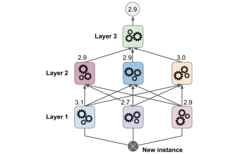
Unfortunately, Scikit-Learn does not support stacking directly, but it is not too hard to roll out your own implementation.

Exercise for Stacking Ensemble

Run the individual classifiers from the previous exercise to make predictions on the validation set, and create a new training set with the resulting predictions: each training instance is a vector containing the set of predictions from all your classifiers for an image, and the target is the image’s class. Train a Random Forest classifier as a blender on this new training set.

import numpy as np
from sklearn.ensemble import RandomForestClassifier, ExtraTreesClassifier
from sklearn.svm import LinearSVC
from sklearn.neural_network import MLPClassifier
from sklearn.ensemble import VotingClassifier
from sklearn.model_selection import train_test_split
import tensorflow as tf
from sklearn.metrics import accuracy_score

(X_train_val, y_train_val), (X_test, y_test) = tf.keras.datasets.mnist.load_data()
X_train, X_val, y_train, y_val = train_test_split(X_train_val.reshape(-1,784), y_train_val, test_size=10000, random_state=42)

random_forest_clf = RandomForestClassifier(n_estimators=10, random_state=42)
extra_trees_clf = ExtraTreesClassifier(n_estimators=10, random_state=42)
svm_clf = LinearSVC(random_state=42)
mlp_clf = MLPClassifier(random_state=42)

estimators = [random_forest_clf, extra_trees_clf, svm_clf, mlp_clf]
for estimator in estimators:
    print("Training the", estimator)
    estimator.fit(X_train, y_train)
    
print([estimator.score(X_val, y_val) for estimator in estimators])
#[0.9446, 0.9507, 0.8626, 0.9576]
#The linear SVM is far outperformed by the other classifiers. 

X_val_predictions = np.empty((len(X_val), len(estimators)), dtype=np.float32)

for index, estimator in enumerate(estimators):
    X_val_predictions[:, index] = estimator.predict(X_val)
    
print(X_val_predictions)
# [[7. 7. 7. 7.]
#  [3. 3. 3. 3.]
#  [8. 8. 8. 8.]
#  ...
#  [9. 9. 9. 9.]
#  [8. 8. 2. 8.]
#  [2. 3. 5. 1.]]

rnd_forest_blender = RandomForestClassifier(n_estimators=200, oob_score=True, random_state=42)
rnd_forest_blender.fit(X_val_predictions, y_val)

print(rnd_forest_blender.oob_score_)
#0.9622

You could fine-tune this blender or try other types of blenders (e.g., an MLPClassifier), then select the best one using cross-validation, as always.

Now let’s evaluate the ensemble on the test set. For each image in the test set, make predictions with all your classifiers, then feed the predictions to the blender to get the ensemble’s predictions.

X_test_predictions = np.empty((len(X_test), len(estimators)), dtype=np.float32)

for index, estimator in enumerate(estimators):
    X_test_predictions[:, index] = estimator.predict(X_test.reshape(-1, 784))
    
y_pred = rnd_forest_blender.predict(X_test_predictions)
print(accuracy_score(y_test, y_pred))
#0.9578

Pittfalls of Ensemble Learning

1. Ensemble methods are usually computationally expensive. Therefore, they add learning time and memory constrains to the problem.
2. The model that is closest to the true data generating process will always be best and will beat most ensemble methods. So if the data come from a linear process, linear models will be much superior to ensemble models.
3. Ensemble models suffer from lack of interpretability and explainability.
4. There are several ensemble methods, each with its own advantages/weaknesses. Which one to use and then depends on the problem at hand. For example, if you have models with high variance (they over-fit your data), then you are likely to benefit from using bagging. If you have biased models, it is better to combine them with Boosting.

REFERENCES

1. https://stats.stackexchange.com/questions/158382/when-should-i-not-use-an-ensemble-classifier
2. https://machinelearningmastery.com/bagging-and-random-forest-ensemble-algorithms-for-machine-learning/
3. https://chrisalbon.com/machine_learning/trees_and_forests/adaboost_classifier/
4. https://www.toptal.com/machine-learning/ensemble-methods-machine-learning
5. https://sebastianraschka.com/Articles/2014_ensemble_classifier.html
6. http://datajango.com/heterogeneous-ensemble-learning-hard-voting-soft-voting/
7. https://www.stat.berkeley.edu/~breiman/randomforest2001.pdf
8. Aurélien Géron, Hands-on Machine Learning with Scikit-Learn, Keras, and TensorFlow, 2nd Edition, O’Reilly Media, Inc., https://www.oreilly.com/library/view/hands-on-machine-learning/9781492032632/
9. Michel Ballings’ BZAN 554: Customer Analytics course notes at University of Tennessee, Knoxville, http://ballings.co/
10. https://www.stat.berkeley.edu/~breiman/RandomForests/cc_home.htm#ooberr