on
21 mins to read.
Naive Bayes Classifier example by hand and how to do in Scikit-Learn
Naive Bayes Classifier
A Naive Bayes classifier is a probabilistic non-linear machine learning model that’s used for classification task. The crux of the classifier is based on the Bayes theorem.
\[P(A \mid B) = \frac{P(A, B)}{P(B)} = \frac{P(B\mid A) \times P (A)}{P(B)}\]NOTE: Generative Classifiers learn a model of the joint probability $p(x, y)$, of the inputs $x$ and the output $y$, and make their predictions by using Bayes rule to calculate $p(y \mid x)$ and then picking the most likely $y$. Discriminative classifers model the posterior $p(y \mid x)$ directly or learn a direct map from inputs $x$ to the class labels. There are several compelling reasons for using discriminative rather than generative classifiers, one of which, succinctly articulated by Vapnik, is that “one should solve the classification problem directly, and never solve a more general problem as an intermediate step (such as modelling $p(y \mid x)$)”. Indeed, leaving aside computational issues and matters such as handling missing data, the prevailing consensus seems to be that the discriminative classifiers are almost always preferred to generative ones.
It is termed as ‘Naive’ because it assumes independence between every pair of feature in the data. That is presence of one particular feature does not affect the other. Bayes’ rule without the independence assumption is called a bayesian network.
Let $(x_{1}, x_{2},…, x_{p})$ be a feature vector and $y$ be the class label corresponding to this feature vector. Applying Bayes’ theorem,
\[P(y \mid X) = \frac{P(X, y)}{P(X)} = \frac{P(X\mid y) \times P (y)}{P(X)}\]where $X$ is given as $X = (x_{1}, x_{2}, …, x_{p})$. By substituting for X and expanding using the chain rule we get,
\[P(y \mid x_{1}, x_{2},..., x_{p}) = \frac{P(x_{1}, x_{2},..., x_{p}, y)}{P(x_{1}, x_{2},..., x_{p})} = \frac{P(x_{1}, x_{2},..., x_{p}\mid y) \times P (y)}{P(x_{1}, x_{2},..., x_{p})}\]Since, $(x_{1}, x_{2},…, x_{p})$ are independent of each other,
\[P(y \mid x_{1}, x_{2},..., x_{p}) = \frac{P (y) \times \prod_{i=1}^{p} P(x_{i} \mid y)}{\prod_{i=1}^{p} P(x_{i})}\]For all entries in the dataset, the denominator does not change, it remains constant. Therefore, the denominator can be removed and a proportionality can be introduced.
\[P(y \mid x_{1}, x_{2},..., x_{p}) \propto P (y) \times \prod_{i=1}^{p} P(x_{i} \mid y)\]In our case, the response variable ($y$) has only two outcomes, binary (e.g., yes or no / positive or negative). There could be cases where the classification could be multivariate.
To complete the specification of our classifier, we adopt the MAP (Maximum A Posteriori) decision rule, which assigns the label to the class with the highest posterior.
\[\hat{y} = p(X, y) = p(y, x_{1}, x_{2},..., x_{p}) = \operatorname*{argmax}_{k \in \{1,2, ...,K\}} P (y) \times \prod_{i=1}^{p} P(x_{i} \mid y)\]We calculate probability for all ‘K’ classes using the above function and take one with the maximum value to classify a new point belongs to that class.
Types of NB Classifier
-
Multinomial Naive Bayes: It is used for discrete counts. This is mostly used for document classification problem, i.e whether a document belongs to the category of sports, politics, technology etc. The features/predictors used by the classifier are the frequency of the words present in the document.
-
Gaussian Naive Bayes: It is used in classification and it assumes that the predictors/features take up a continuous value and are not discrete, we assume that these values are sampled from a gaussian distribution (follow a normal distribution). The parameters of the Gaussian are the mean and variance of the feature values. Since the way the values are present in the dataset changes, the formula for conditional probability changes to:
\[P(x_{i} \mid y) = \frac{1}{\sqrt{2 \pi \sigma^{2}_{y}}} \exp \left(- \frac{\left(x_{i} - \mu_{y}\right)^{2}}{2\sigma^{2}_{y}} \right)\]If continuous features do not have normal distribution, we should use transformation or different methods to convert it in normal distribution.
Alternatively, a continuous feature could be discretized by binning its values, but doing so throws away information, and results could be sensitive to the binning scheme.
-
Bernoulli Naive Bayes: This is similar to the multinomial naive bayes. In the multivariate Bernoulli event model, features are independent booleans (binary variables) describing inputs, for example if a word occurs in the text or not.
\[P(x_{1}, x_{2},..., x_{p}\mid y) = \prod_{i=1}^{p} p_{ki}^{x_{i}} (1-p_{ki})^{(1-x_{i})}\]where where $p_{ki}$ is the probability of class k generating the term $x_{i}$.
Using one of the three common distributions is not mandatory; for example, if a real-valued variable is known to have a different specific distribution, such as exponential, then that specific distribution may be used instead. If a real-valued variable does not have a well-defined distribution, such as bimodal or multimodal, then a kernel density estimator can be used to estimate the probability distribution instead.
Advantages
-
It is really easy to implement and often works well. Training is quick, and consists of computing the priors and the likelihoods. Prediction on a new data point is also quick. First calculate the posterior for each class. Then apply the MAP decision rule: the label is the class with the maximum posterior.
-
CPU usage is modest: there are no gradients or iterative parameter updates to compute, since prediction and training employ only analytic formulae.
-
The Naive Bayes classifier does not converge at all. Rather than learning its parameters by iteratively tweaking them to minimize a loss function using gradient descent like the vast majority of machine learning models, the Naive Bayes classifier learns it parameters by explicitly calculating them. The Naive Bayes classifier trains faster than logistic regression for this reason; the simple counting the calculation of its parameters consists run much faster than gradient decent.
-
The memory requirement is very low because these operations do not require the whole data set to be held in RAM at once.
-
It is often a good first thing to try. For problems with a small amount of training data, it can achieve better results than other classifiers, thanks to Occam’s Razor because it has a low propensity to overfit.
-
Easily handles missing feature values — by re-training and predicting without that feature! (See this quora answer)
-
As new data becomes available, it can be relatively straightforward to use this new data with the old data to update the estimates of the parameters for each variable’s probability distribution. This allows the model to easily make use of new data or the changing distributions of data over time.
-
It can handle numeric and categorical variables very well.
Disadvantages
-
Ensembling, boosting, bagging will not work here since the purpose of these methods is to reduce variance. Naive Bayes has no variance to minimize.
-
It is important to note that categorical variables need to be factors with the same levels in both training and new data (testing dataset). This can be problematic in a predictive context if the new data obtained in the future does not contain all the levels, meaning it will be unable to make a prediction. This is often known as “Zero Frequency”. To solve this, we can use a smoothing technique. One of the simplest smoothing techniques is called Laplace smoothing.
-
Another limitation of Naive Bayes is the assumption of independent predictors. In real life, it is almost impossible that we get a set of predictors which are completely independent. Additionally, the performance of the algorithm degrades, the more dependent the input variables happen to be because Naive Bayes algorithm ignores correlation among the features, which induces bias and hence reduces variance.
-
It cannot incorporate feature interactions.
-
Performance is sensitive to skewed data — that is, when the training data is not representative of the class distributions in the overall population. In this case, the prior estimates will be incorrect.
-
The calculation of the independent conditional probability for one example for one class label involves multiplying many probabilities together, one for the class and one for each input variable. As such, the multiplication of many small numbers together can become numerically unstable, especially as the number of input variables increases. To overcome this problem, it is common to change the calculation from the product of probabilities to the sum of log probabilities. For example:
\[P(y \mid x_{1}, x_{2},..., x_{p}) \propto log(P (y)) + \sum_{i=1}^{p} log(P(x_{i} \mid y))\]Calculating the natural logarithm of probabilities has the effect of creating larger (negative) numbers and adding the numbers together will mean that larger probabilities will be closer to zero. The resulting values can still be compared and maximized to give the most likely class label. This is often called the log-trick when multiplying probabilities.
An Example by hand

Let’s find the class of this test record:
\[X=(Refund = No, Married, Income = 120K)\]- For income variable when Evade = No:
- Sample mean: 110
- Sample Variance = 2975
- For income variable when Evade = Yes:
- Sample mean: 90
- Sample Variance = 25
Therefore, we can compute the likelihoods of a continuous feature vector:
\[P(Income = 120 \mid Evade = No) = \frac{1}{\sqrt{2 \times \pi \times 2975}} \exp \left(- \frac{\left(120 - 110\right)^{2}}{2 \times 2975} \right) = 0.007192295359419549\] \[P(Income = 120 \mid Evade = Yes) = \frac{1}{\sqrt{2 \times \pi \times 25}} \exp \left(- \frac{\left(120 - 90\right)^{2}}{2 \times 25} \right) = 1.2151765699646572e^{-9}\]In order to compute the class-conditional probability (posterior probability) of a sample, we can simply form the product of the likelihoods from the different feature subsets:
\[\begin{split} P(X \mid Evade = No) &= P(Refund = No \mid Evade = No) \times P(Married \mid Evade = No) \times P(Income = 120K \mid Evade = No) \\ &= \frac{4}{7} \times \frac{4}{7} \times 0.007192295359419549 \\ &= 0.0023485046071574033 \end{split}\] \[\begin{split} P(X \mid Evade = Yes) &= P(Refund = No \mid Evade = Yes) \times P(Married \mid Evade = Yes) \times P(Income = 120K \mid Evade = Yes) \\ &= \frac{3}{3} \times 0 \times 1.2151765699646572e^{-9} \\ &= 0 \end{split}\]Since $P(X \mid Evade = No) \times P(Evade = No) > P(X \mid Evade = Yes) \times P(Evade = Yes)$, therefore, $P(No \mid X) > P(Yes \mid X)$, the class of this instance is then No.
NB Classifier for Text Classification
Let’s now give an example of text classification using Naive Bayes method. Although this method is a two-class problem, the same approaches are applicable ot multi-class setting.
Let’ssay we have a set of reviews (document) and its classes:
| Document | Text | Class |
|---|---|---|
| 1 | I loved the movie | + |
| 2 | I hated the movie | - |
| 3 | a great movie. good movie | + |
| 4 | poor acting | - |
| 5 | great acting. a good movie | + |
Prior to fitting the model and using machine learning algorithm for training, we need to think about how to best represent a text document as a feature vector. A commonly used model in Natural Language Processing (NLP) is so-called bag of words model.
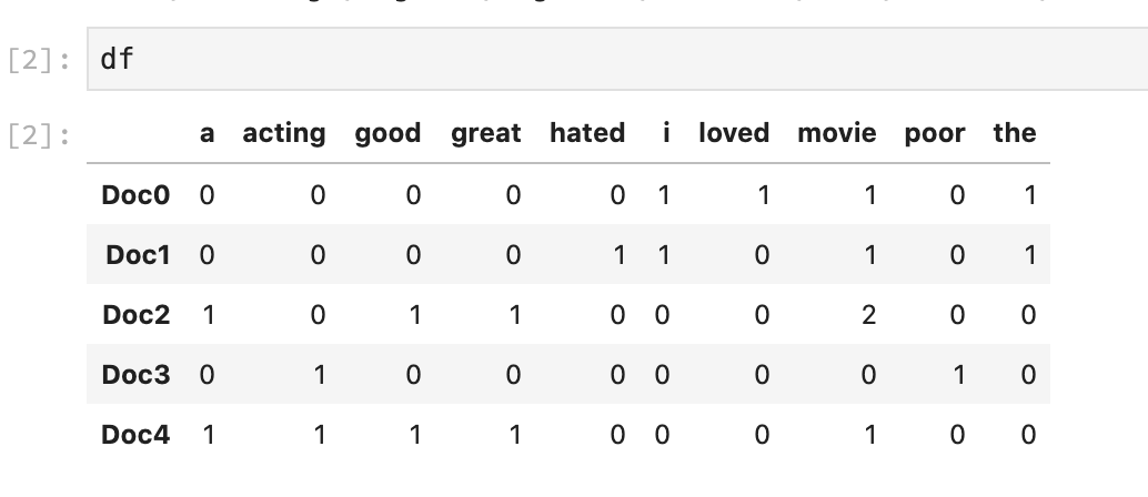
The idea behind this model is really simple. First step is the creating of the vocabulary - the collection of all different words that occur in the training set. For our example, vocabulari, which consists of 10 unique words could be written as:
< I, loved, the, movie, hated, a, great, poor, acting, good >
Using tokenization which is general process of breaking down a text corpus into individual elements that serve as input for various NLP methods, Usually, tokenization is accompanied by other optional processing steps such as removal of stop words and punctuation characters, stemming or lemmetizing and construction of n-grams.
Using Python, let’s convert the documents into feature sets, where the attributes are possible words and the values are number of times a word occurs in the given document.
import numpy as np
import pandas as pd
from sklearn.feature_extraction.text import CountVectorizer
corpus = ['I loved the movie', 'I hated the movie', 'a great movie. good movie', 'poor acting', 'great acting. a good movie']
vectorizer = CountVectorizer(analyzer = "word",
                             lowercase=True,
                             tokenizer = None,
                             preprocessor = None,
                             stop_words = None,
                             max_features = 5000,
                             token_pattern='[a-zA-Z0-9$&+,:;=?@#|<>^*()%!-]+')
#you can change the pattern for tokens. Here, I accepted "I" and "a" as tokens too!

# convert the documents into a document-term matrix
wm = vectorizer.fit_transform(corpus)
print(wm.todense())
# [[0 0 0 0 0 1 1 1 0 1]
#  [0 0 0 0 1 1 0 1 0 1]
#  [1 0 1 1 0 0 0 2 0 0]
#  [0 1 0 0 0 0 0 0 1 0]
#  [1 1 1 1 0 0 0 1 0 0]]

#shape of count vector: 5 documents and 10 unique words (columns)!
print(wm.shape)
#(5, 10)

# show resulting vocabulary; the numbers are not counts, they are the position in the sparse vector
vocabulary = vectorizer.vocabulary_
print(vocabulary)
#{'i': 5, 'loved': 6, 'the': 9, 'movie': 7, 'hated': 4, 'a': 0, 'great': 3, 'good': 2, 'poor': 8, 'acting': 1}

tokens = vectorizer.get_feature_names()
print(tokens)
#['a', 'acting', 'good', 'great', 'hated', 'i', 'loved', 'movie', 'poor', 'the']

# create an index for each row
doc_names = ['Doc{:d}'.format(idx) for idx, _ in enumerate(wm)]
df = pd.DataFrame(data=wm.toarray(), index=doc_names,
                  columns=tokens)
Let’s look at the probabilities per outcome (class, + or -):
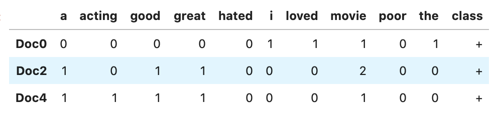
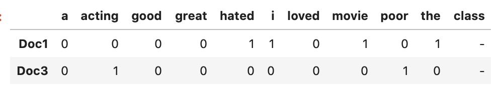
df['class'] = ['+', '-', '+', '-','+']
df[df['class'] == '+']
df[df['class'] == '-']
Let’s do positively-classified documents, first. Since we have 5 documents and 3 of them are classified positive (+):
Then we need to computer some conditional probabilities, $P( I \mid + )$, $P( loved \mid + )$, $P( the \mid + )$, $P( movie \mid + )$, $P( a \mid + )$, $P( great \mid + )$, $P( acting \mid + )$, $P( good \mid + )$, $P( poor \mid + )$, $P( hated \mid + )$.
Let $n$ be the number of total words in + case, which is 14. $n_{k}$ is the number of times that the word $k$ occurs in these + cases. Then, we can compute the probability of each word given it is classified as positive, as in the following:
where $\mid \text{vocabulary} \mid$ is the size of the vocabulary.
NOTE: Actually, the main formula is:
\[P( w_{k} \mid +) = \frac{n_{k}}{n}\]since each word has two outcomes, either 0 or 1 (Bernoulli). However, the first formula we talked about is called Laplace smoothing (add-1 - also called as additive smoothing) for Naive bayes algorithm (not to be confused with Laplacian smoothing), for words that do not appear in the training set while we do the training and inference. For example, after training, when we try to predict the class of a new review which contains the word “terrible”, the probability would be:
\[P (w_{\text{terrible}} \mid +) = \frac{0}{14} = 0\]for positive case. This is often known as Zero frequency and we use this smoothing technique to fix the problem.
Let’s now calculate the probabilities we gave above:
\[P( I \mid + ) = \frac{1 + 1}{14 + 10} = 0.0833\] \[P( loved \mid + ) = \frac{1 + 1}{14 + 10} = 0.0833\] \[P( the \mid + ) = \frac{1 + 1}{14 + 10} = 0.0833\] \[P( movie \mid + ) = \frac{4 + 1}{14 + 10} = 0.20833\] \[P( a \mid + ) = \frac{2 + 1}{14 + 10} = 0.125\] \[P( great \mid + ) = \frac{2 + 1}{14 + 10} = 0.125\] \[P( acting \mid + ) = \frac{1 + 1}{14 + 10} = 0.0833\] \[P( good \mid + ) = \frac{2 + 1}{14 + 10} = 0.125\] \[P( poor \mid + ) = \frac{0 + 1}{14 + 10} = 0.0417\] \[P( hated \mid + )= \frac{0 + 1}{14 + 10} = 0.0417\]We can repeat the same step for negative (-) examples:
Now that we have trained our classifier, let’s classify a new sentence according to:
\[V_{NB} = \underset{v_{j} \in V}{\arg\max} \,\,\,P(v_{j}) \sum_{w \in word} P( w \mid v_{j})\]where $v$ stands for value or class!
This is a new sentence: “I hated the poor acting”:
-
if $v_{j} = + $, we will have:
\[P(+)P( I \mid + )P( hated \mid + )P( the \mid + )P( poor \mid + )P( acting \mid + ) = 6.03 \times 10^{-7}\] -
if $v_{j} = - $, we will have:
\[P(-)P( I \mid - )P( hated \mid - )P( the \mid - )P( poor \mid - )P( acting \mid - ) = 1.22 \times 10^{-5}\]
Clearly, this review is a negative (-) review which has the bigger probability.
Additional note about Laplace smoothing technique. In some documents, its formula is given by:
\[\hat{\phi_{i}} = \frac{x_{i} + \alpha}{N + \alpha d},\,\,\,\, i = 1, 2, \dots , d\]where the pseudocount $\alpha > 0$ is the smoothing parameter ($\alpha = 0$ corresponds to no smoothing). Additive smoothing is a type of shrinkage estimator as the resulting estimate will be between the empirical estimate $\frac{x_{i}}{N}$ and the uniform probability $\frac{1}{d}$. Some people argued that $\alpha$ should be 1 (in which case the term add-one smoothing is also used), though in practice smaller values is typically chosen.
DATA: Iris Flower Dataset
# loading libraries
import numpy as np
from sklearn.cross_validation import train_test_split
import pandas as pd
from sklearn.datasets import load_iris

data = load_iris()
X = data['data']
y = data['target']
# split into train and test
X_train, X_test, y_train, y_test = train_test_split(X, y, test_size=0.33, random_state=42)
Gaussian Naive Bayes Classifier in Sci-kit Learn
# Fitting Naive Bayes Classification to the Training set with linear kernel
from sklearn.naive_bayes import GaussianNB
from sklearn.metrics import accuracy_score

GNBclassifier = GaussianNB()
GNBclassifier.fit(X_train, y_train)

# Predicting the Test set results
y_pred_GNB = GNBclassifier.predict(X_test)

# evaluate accuracy
print('\nThe accuracy of Gaussian Naive Bayes Classifier is {}%'.format(accuracy_score(y_test, y_pred_GNB)*100))
#The accuracy of Gaussian Naive Bayes Classifier is 96.0%
Multinomial Naive Bayes Classifier in Sci-kit Learn
Multinomial naive Bayes works similar to Gaussian naive Bayes, however the features are assumed to be multinomially distributed. In practice, this means that this classifier is commonly used when we have discrete data (e.g. movie ratings ranging 1 and 5).
# Load libraries
import numpy as np
from sklearn.naive_bayes import MultinomialNB
from sklearn.feature_extraction.text import CountVectorizer

# Create text
text_data = np.array(['I love Brazil. Brazil!',
                      'Brazil is best',
                      'Germany beats both'])

# Create bag of words
count = CountVectorizer()
bag_of_words = count.fit_transform(text_data)

# Create feature matrix
X = bag_of_words.toarray()
# array([[0, 0, 0, 2, 0, 0, 1],
#        [0, 1, 0, 1, 0, 1, 0],
#        [1, 0, 1, 0, 1, 0, 0]])

# Create target vector
y = np.array([0,0,1])

#Train Multinomial Naive Bayes Classifier
# Create multinomial naive Bayes object with prior probabilities of each class
clf = MultinomialNB(class_prior=[0.25, 0.5])

# Train model
model = clf.fit(X, y)

# Create new observation
new_observation = [[0, 0, 0, 1, 0, 1, 0]]

# Predict new observation's class
model.predict(new_observation)
#array([0])
Naive Bayes fo mixed dataset
Since we have the conditional independence assumption in Naive Bayes, we see that mixing variables is not a problem. Now consider the case where you have a dataset consisting of several features:
- Categorical
- Bernoulli
- Normal
Under the very assumption of using NB, these variables are independent. Consequently, you can do the following:
- Build a NB classifier for each of the categorical data separately, using your dummy variables and a multinomial NB.
- Build a NB classifier for all of the Bernoulli data at once - this is because sklearn’s Bernoulli NB is simply a shortcut for several single-feature Bernoulli NBs.
- Same as 2 for all the normal features.
By the definition of independence, the probability for an instance, is the product of the probabilities of instances by these classifiers.
For aditional details, look here or here or here or here.