Written by MMA
on July 23, 2019
29 mins to read.

Implementing K-means Clustering from Scratch - in Python

K-means Clustering

K-means algorithm is is one of the simplest and popular unsupervised machine learning algorithms, that solve the well-known clustering problem, with no pre-determined labels defined, meaning that we don’t have any target variable as in the case of supervised learning. It is often referred to as Lloyd’s algorithm.

K-means simply partitions the given dataset into various clusters (groups).

K refers to the total number of clusters to be defined in the entire dataset.There is a centroid chosen for a given cluster type which is used to calculate the distance of a given data point. The distance essentially represents the similarity of features of a data point to a cluster type.

You’ll define a target number K, which refers to the number of centroids you need in the dataset. A centroid is the imaginary or real location representing the center of the cluster. These centroids shoud be placed in a cunning way because of different location causes different result. So, the better choice is to place them as much as possible far away from each other.

In other words, the K-means algorithm identifies K number of centroids, and then allocates every data point to the nearest cluster, while keeping the centroids as small as possible. The ‘means’ in the K-means refers to averaging of the data; that is, finding the centroid.

Every data point is allocated to each of the clusters through reducing the in-cluster sum of squares. Once the algorithm has been run and the groups are defined, any new data can be easily assigned to the correct group.

In K-means, each cluster is described by a single mean, or centroid (hard clustering), so as not to confuse this model with an actual probabilistic model. There is no underlying probability model in K-means. The goal is to group data into K clusters. K-means (and some other clustering methods) have hard boundaries, meaning a data point either belongs to that cluster or it does not. On the other hand, clustering methods such as Gaussian Mixture Models (GMM) have soft boundaries (soft clustering), where data points can belong to multiple cluster at the same time but with different degrees of belief. e.g. a data point can have a $60\%$ of belonging to cluster $1$, $40\%$ of belonging to cluster $2$. Additionally, in probabilistic clustering, clusters can overlap (K-means doesn’t allow this).

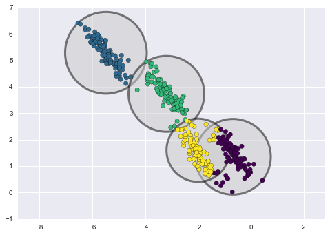
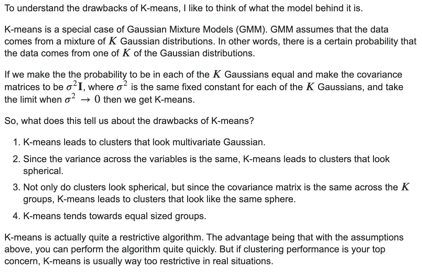
An important observation for K-means is that the cluster models must be circular in 2D (or spherical in 3D or higher, i.i.d. Gaussian). In other words, K-means requires that each blob be a fixed size and completely symmetrical. K-means has no built-in way of accounting for oblong or elliptical clusters. When clusters are non-circular, trying to fit circular clusters would be a poor fit. This results in a mixing of cluster assignments where the resulting circles overlap.

Unfortunately, K-means will not work for non-spherical clusters like these:

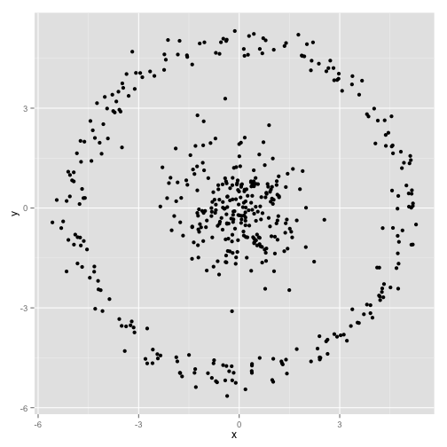
These two disadvantages of K-means—its lack of flexibility in cluster shape and lack of probabilistic cluster assignment—mean that for many datasets (especially low-dimensional datasets) it may not perform as well as you might hope. K-means is also very sensitive to outliers and noise in the dataset.

K-means is a widely used method in cluster analysis. One might easily think that this method does NOT require ANY assumptions, i.e., give me a data set and a pre-specified number of clusters, K, then I just apply this algorithm which minimize the total within-cluster square error (intra-cluster variance). See “Constraints of the algorithm” section for more details!

When to use?

This is a versatile algorithm that can be used for any type of grouping. Some examples of use cases are:

Image Segmentation
Clustering Gene Segmentation Data
News Article Clustering
Clustering Languages
Species Clustering
Anomaly Detection

Algorithm

The Κ-means clustering algorithm uses iterative refinement to produce a final result. The algorithm inputs are the number of clusters Κ and the data set. The data set is a collection of features for each data point.

Step 1

The algorithms starts with initial estimates for the Κ centroids, which can either be randomly generated or randomly selected from the data set. Random initialization is not an efficient way to start with, as sometimes it leads to increased numbers of required clustering iterations to reach convergence, a greater overall runtime, and a less-efficient algorithm overall. So there are many techniques to solve this problem like K-means++ etc.

We randomly pick K cluster centers(centroids). Let’s assume these are $c_1, c_2, …, c_K$, and we can say that;

\[C = {c_1, c_2,..., c_K}\]

where $C$ is the set of all centroids.

Step 2

Each centroid defines one of the clusters. In this step, each data point is assigned to its nearest centroid, based on the squared Euclidean distance. More formally, if $c_{i}$ is the collection of centroids in set $C$, then each data point $x$ is assigned to a cluster based on

\[\underset{c_i \in C}{\arg\min} \; dist(c_i,x)^2\]

where $dist( \cdot )$ is the standard (L2) Euclidean distance. Let the set of data point assignments for each ith cluster centroid be $S_{i}$. Note that the distance function in the cluster assignment step can be chosen specifically for your problem, and is arbitrary.

Step 3

In this step, the centroids are recomputed. This is done by taking the mean of all data points assigned to that centroid’s cluster.

\[c_i=\frac{1}{\lvert S_i \rvert}\sum_{x_i \in S_i} x_i\]

where $S_{i}$ is the set of all points assigned to the $i$th cluster.

Step 4

The algorithm iterates between steps one and two until a stopping criteria is met (i.e., no data points change clusters, the sum of the distances is minimized, or some maximum number of iterations is reached).

The best number of clusters K leading to the greatest separation (distance) is not known as a priori and must be computed from the data. The objective of K-Means clustering is to minimize total intra-cluster variance, or, the squared error function:

NOTE: Unfortunately, although the algorithm is guaranteed to converge, it may not converge to the right solution (i.e., it may converge to a local optimum, not necessarily the best possible outcome). This highly depends on the centroid initialization. As a result, the computation is often done several times, with different initializations of the centroids. One method to help address this issue is the K-means++ initialization scheme, which has been implemented in scikit-learn (use the init='k-means++' parameter). This initializes the centroids to be (generally) distant from each other, leading to probably better results than random initialization. One idea for initializing K-means is to use a farthest-first traversal on the data set, to pick K points that are far away from each other. However, this is too sensitive to outliers. But, K-means++ procedure picks the K centers one at a time, but instead of always choosing the point farthest from those picked so far, choose each point at random, with probability proportional to its squared distance from the centers chosen already.

NOTE: The computational complexity of the algorithm is generally linear with regards to the number of instances, the number of clusters and the number of dimensions. However, this is only true when the data has a clustering structure. If it does not, then in the worst case scenario the complexity can increase exponentially with the number of instances. In practice, however, this rarely happens, and K-means is generally one of the fastest clustering algorithms.

Choosing the Value of K

Determining the right number of clusters in a data set is important, not only because some clustering algorithms like k-means requires such a parameter, but also because the appropriate number of clusters controls the proper granularity of cluster analysis. determining the number of clusters is far from easy, often because the right number is ambiguous. The interpretations of the number of clusters often depend on the shape and scale of the distribution in a data set, as well as the clustering resolution required by a user. There are many possible ways to estimate the number of clusters. Here, we briefly introduce some simple yet popularly used and effective methods.

We often know the value of K. In that case we use the value of K. In general, there is no method for determining exact value of K.

A simple experienced method is to set the number of clusters to about $\sqrt{n/2}$ for a data set of $n$ points. In expectation, each cluster has $\sqrt{2n}$ points. Another approach is the Elbow Method. We run the algorithm for different values of K (say K = 1 to 10) and plot the K values against WCSSE (Within Cluster Sum of Squared Errors). WCSS is also called “inertia”. Then, select the value of K that causes sudden drop in the sum of squared distances, i.e., for the elbow point as shown in the figure.

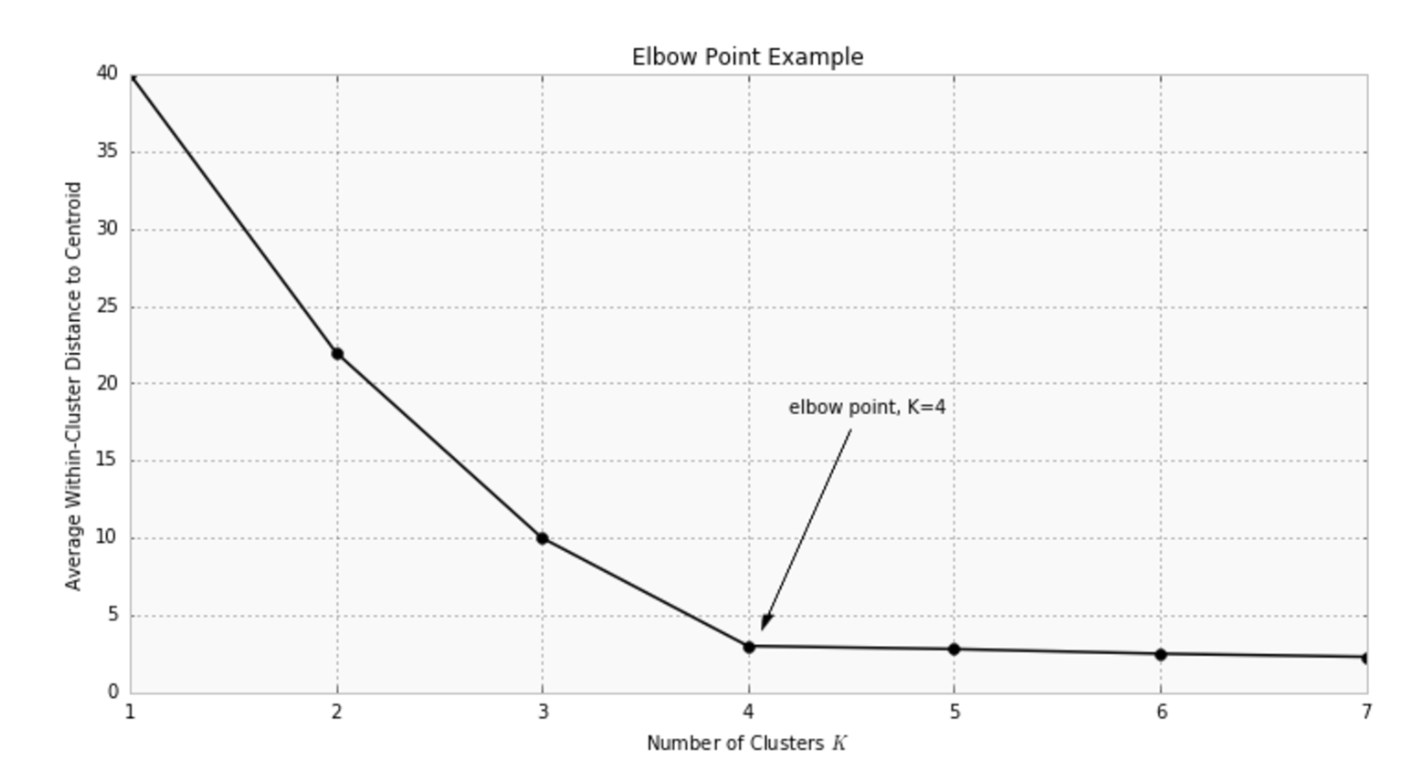
HOWEVER, it is important to note that inertia heavily relies on the assumption that the clusters are convex (of spherical shape).

A number of other techniques exist for validating K, including cross-validation, information criteria, the information theoretic jump method, the silhouette method (we want to have high silhouette coefficient for the number of clusters we want to use), and the G-means algorithm.

import numpy as np
import pandas as pd
import matplotlib.pyplot as plt
plt.style.use('ggplot')

from sklearn.datasets import make_blobs
from sklearn.preprocessing import MinMaxScaler
from sklearn.cluster import KMeans
from sklearn.metrics import silhouette_score, davies_bouldin_score,v_measure_score

n_features = 4
n_cluster = 5
cluster_std = 1.2
n_samples = 200

data = make_blobs(n_samples=n_samples,n_features=n_features,centers=n_cluster,cluster_std=cluster_std)
data[0].shape
#(200, 4)

scaler = MinMaxScaler()
X_scaled=scaler.fit_transform(data[0])
y = data[1]

km_scores= []
km_silhouette = []
vmeasure_score =[]
db_score = []

for i in range(2,12):
    km = KMeans(n_clusters=i, random_state=0).fit(X_scaled)
    preds = km.predict(X_scaled)
    
    print("Score for number of cluster(s) {}: {}".format(i,km.score(X_scaled)))
    km_scores.append(-km.score(X_scaled))
    
    silhouette = silhouette_score(X_scaled,preds)
    km_silhouette.append(silhouette)
    print("Silhouette score for number of cluster(s) {}: {}".format(i,silhouette))
    
    db = davies_bouldin_score(X_scaled,preds)
    db_score.append(db)
    print("Davies Bouldin score for number of cluster(s) {}: {}".format(i,db))
    
    v_measure = v_measure_score(y,preds)
    vmeasure_score.append(v_measure)
    print("V-measure score for number of cluster(s) {}: {}".format(i,v_measure))
    print("-"*70)
    
# Score for number of cluster(s) 2: -31.3569004250751
# Silhouette score for number of cluster(s) 2: 0.533748527011396
# Davies Bouldin score for number of cluster(s) 2: 0.5383728596874554
# V-measure score for number of cluster(s) 2: 0.47435098761403227
# ----------------------------------------------------------------------
# Score for number of cluster(s) 3: -14.975981331453639
# Silhouette score for number of cluster(s) 3: 0.595652250150026
# Davies Bouldin score for number of cluster(s) 3: 0.536655881702941
# V-measure score for number of cluster(s) 3: 0.7424834172925047
# ----------------------------------------------------------------------
# Score for number of cluster(s) 4: -5.590224681322909
# Silhouette score for number of cluster(s) 4: 0.6811747762083824
# Davies Bouldin score for number of cluster(s) 4: 0.4571807219192957
# V-measure score for number of cluster(s) 4: 0.9057460992755187
# ----------------------------------------------------------------------
# Score for number of cluster(s) 5: -2.6603963145009493
# Silhouette score for number of cluster(s) 5: 0.7014652472967188
# Davies Bouldin score for number of cluster(s) 5: 0.4361514672175016
# V-measure score for number of cluster(s) 5: 1.0
# ----------------------------------------------------------------------
# Score for number of cluster(s) 6: -2.4881557936377554
# Silhouette score for number of cluster(s) 6: 0.6325414350157488
# Davies Bouldin score for number of cluster(s) 6: 0.7063862889372524
# V-measure score for number of cluster(s) 6: 0.9634327805669886
# ----------------------------------------------------------------------
# Score for number of cluster(s) 7: -2.3316753100814296
# Silhouette score for number of cluster(s) 7: 0.5322227493562578
# Davies Bouldin score for number of cluster(s) 7: 1.0188824098593388
# V-measure score for number of cluster(s) 7: 0.9218233659260291
# ----------------------------------------------------------------------
# Score for number of cluster(s) 8: -2.18382508736358
# Silhouette score for number of cluster(s) 8: 0.42724909671055145
# Davies Bouldin score for number of cluster(s) 8: 1.2282408117318253
# V-measure score for number of cluster(s) 8: 0.8868684126315897
# ----------------------------------------------------------------------
# Score for number of cluster(s) 9: -2.0869677530855695
# Silhouette score for number of cluster(s) 9: 0.3368676415036809
# Davies Bouldin score for number of cluster(s) 9: 1.4026173756052418
# V-measure score for number of cluster(s) 9: 0.8563175291018919
# ----------------------------------------------------------------------
# Score for number of cluster(s) 10: -1.9980361222182945
# Silhouette score for number of cluster(s) 10: 0.21171522762641234
# Davies Bouldin score for number of cluster(s) 10: 1.6059328832470423
# V-measure score for number of cluster(s) 10: 0.8264924248537714
# ----------------------------------------------------------------------
# Score for number of cluster(s) 11: -1.8921797505850377
# Silhouette score for number of cluster(s) 11: 0.29941004236481095
# Davies Bouldin score for number of cluster(s) 11: 1.363170543240617
# V-measure score for number of cluster(s) 11: 0.8213630277489044
# ----------------------------------------------------------------------

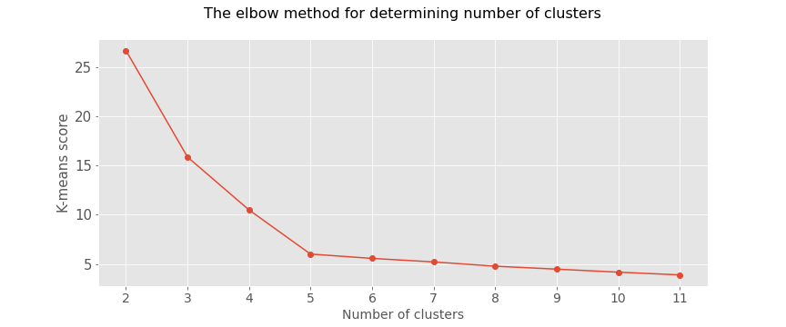
plt.figure(figsize=(12,5))
plt.title("The elbow method for determining number of clusters\n",fontsize=16)
plt.plot([i for i in range(2,12)],km_scores, marker = 'o')
plt.grid(True)
plt.xlabel("Number of clusters",fontsize=14)
plt.ylabel("K-means score",fontsize=15)
plt.xticks([i for i in range(2,12)],fontsize=14)
plt.yticks(fontsize=15)
plt.savefig('the_elbow_method.png')
plt.show()

plt.figure(figsize=(12,5))
plt.plot([i for i in range(2,12)],vmeasure_score, marker = 'o')
plt.grid(True)
plt.xlabel('Number of Clusters',fontsize=14)
plt.title("V-measure score")
plt.savefig('v_measure_score.png')
plt.show()

plt.figure(figsize=(12,5))
plt.title("The silhouette coefficient method \nfor determining number of clusters\n",fontsize=16)
plt.plot([i for i in range(2,12)], km_silhouette, marker = 'o')
plt.grid(True)
plt.xlabel("Number of clusters",fontsize=14)
plt.ylabel("Silhouette score",fontsize=15)
plt.xticks([i for i in range(2,12)],fontsize=14)
plt.yticks(fontsize=15)
plt.savefig('the_silhouette_coefficient_method.png')
plt.show()

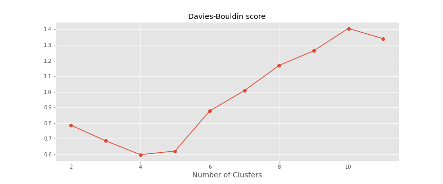
plt.figure(figsize=(12,5))
plt.plot([i for i in range(2,12)], db_score, marker = 'o')
plt.grid(True)
plt.xlabel('Number of Clusters',fontsize=14)
plt.title("Davies-Bouldin score")
plt.savefig('davies_bouldin_score.png')
plt.show()

In addition, monitoring the distribution of data points across groups provides insight into how the algorithm is splitting the data for each K. Some researchers also use Hierarchical clustering first to create dendrograms and identify the distinct groups from there.

Constraints of the algorithm

Only numerical data can be used. Generally K-means works best for 2 dimensional numerical data. Visualization is possible in 2D or 3D data. But in reality there are always multiple features to be considered at a time. However, we must be careful about curse of dimensionality. Any more than few tens of dimensions mean that distance interpretation is not obvious and must be guarded against. Appropriate dimensionality reduction techniques and distance measures must be used.

K-Means clustering is prone to initial seeding i.e. random initialization of centroids which is required to kick-off iterative clustering process. Bad initialization may end up getting bad clusters. Leader Algorithm can be used.

The standard K-means algorithm isn’t directly applicable to categorical data, for various reasons. The sample space for categorical data is discrete, and doesn’t have a natural origin. A Euclidean distance function on such a space is not really meaningful. However, the clustering algorithm is free to choose any distance metric / similarity score. Euclidean is the most popular. But any other metric can be used that scales according to the data distribution in each dimension/attribute, for example the Mahalanobis metric.

The use of Euclidean distance as the measure of dissimilarity can also make the determination of the cluster means non-robust to outliers and noise in the data.

Inertia is not a normalized metric: we just know that lower values are better and zero is optimal. But in very high-dimensional spaces, Euclidean distances tend to become inflated (this is an instance of the so-called “curse of dimensionality”). Running a dimensionality reduction algorithm such as Principal component analysis (PCA) prior to k-means clustering can alleviate this problem and speed up the computations.

Categorical data (i.e., category labels such as gender, country, browser type) needs to be encoded (e.g., one-hot encoding for nominal categorical variable or label encoding for ordinal categorical variable) or separated in a way that can still work with the algorithm, which is still not perfectly right. There’s a variation of K-means known as K-modes, introduced in this paper by Zhexue Huang, which is suitable for categorical data.

K-Means does not behave very well when the clusters have varying sizes, different densities, or non-spherical shapes. In that case, one can use Mixture models using EM algorithm or Fuzzy K-means (every object belongs to every cluster with a membership weight that is between 0 (absolutely does not belong) and 1 (absolutely belongs). which both allow soft assignments. As a matter of fact, K-means is special variant of the EM algorithm with the assumption that the clusters are spherical. EM algorithm also starts with random initializations, it is an iterative algorithm, it has strong assumptions that the data points must fulfill, it is sensitive to outliers, it requires prior knowledge of the number of desired clusters. The results produced by EM are also non-reproducible.

The above paragraph shows the drawbacks of this algorithm. K-means assumes the variance of the distribution of each attribute (variable) is spherical; all variables have the same variance; the prior probability for all K clusters is the same, i.e., each cluster has roughly equal number of observations. If any one of these 3 assumptions are violated, then K-means will fail. This Stackoverflow answer explains perfectly!

It is important to scale the input features before you run K-Means, or else the clusters may be very stretched, and K-Means will perform poorly. Scaling the features does not guarantee that all the clusters will be nice and spherical, but it generally improves things.

K-Means clustering just cannot deal with missing values. Any observation even with one missing dimension must be specially handled. If there are only few observations with missing values then these observations can be excluded from clustering. However, this must have equivalent rule during scoring about how to deal with missing values. Since in practice one cannot just refuse to exclude missing observations from segmentation, often better practice is to impute missing observations. There are various methods available for missing value imputation but care must be taken to ensure that missing imputation doesn’t distort distance calculation implicit in k-Means algorithm. For example, replacing missing age with -1 or missing income with 999999 can be misleading!

Clustering analysis is not negatively affected by heteroscedasticity but the results are negatively impacted by multicollinearity of features/ variables used in clustering as the correlated feature/ variable will carry extra weight on the distance calculation than desired.

K-means has no notion of outliers, so all points are assigned to a cluster even if they do not belong in any. In the domain of anomaly detection, this causes problems as anomalous points will be assigned to the same cluster as “normal” data points. The anomalous points pull the cluster centroid towards them, making it harder to classify them as anomalous points.

K-Means clustering algorithm might converse on local minima which might also correspond to the global minima in some cases but not always. Therefore, it’s advised to run the K-Means algorithm multiple times before drawing inferences about the clusters. However, note that it’s possible to receive same clustering results from K-means by setting the same seed value for each run. But that is done by simply making the algorithm choose the set of same random number for each run.

DATA: Iris Flower Dataset

import numpy as np
from sklearn.datasets import load_iris
import pandas as pd
import matplotlib.pyplot as plt
from sklearn.cluster import KMeans
%matplotlib inline

data = load_iris()
X = data['data']
y = data['target']

# Number of training data
n = X.shape[0]
# Number of features in the data
c = X.shape[1]

# Plot the data
colors=['orange', 'blue', 'green']
for i in range(n):
    plt.scatter(X[i, 0], X[i,1], s=7, color = colors[int(y[i])])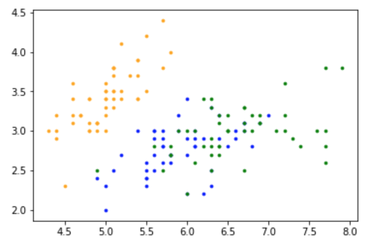

K-means in Sci-kit Learn

Kmean = KMeans(n_clusters=3)
Kmean.fit(X)
centers = Kmean.cluster_centers_
# array([[5.006     , 3.418     , 1.464     , 0.244     ],
#        [5.9016129 , 2.7483871 , 4.39354839, 1.43387097],
#        [6.85      , 3.07368421, 5.74210526, 2.07105263]])

# Plot the data
colors=['orange', 'blue', 'green']
for i in range(n):
    plt.scatter(X[i, 0], X[i,1], s=7, color = colors[int(y[i])])
plt.scatter(centers[:,0], centers[:,1], marker='*', c='g', s=150)

y_pred_clusters = Kmean.labels_
# array([1, 1, 1, 1, 1, 1, 1, 1, 1, 1, 1, 1, 1, 1, 1, 1, 1, 1, 1, 1, 1, 1,
#        1, 1, 1, 1, 1, 1, 1, 1, 1, 1, 1, 1, 1, 1, 1, 1, 1, 1, 1, 1, 1, 1,
#        1, 1, 1, 1, 1, 1, 2, 2, 0, 2, 2, 2, 2, 2, 2, 2, 2, 2, 2, 2, 2, 2,
#        2, 2, 2, 2, 2, 2, 2, 2, 2, 2, 2, 0, 2, 2, 2, 2, 2, 2, 2, 2, 2, 2,
#        2, 2, 2, 2, 2, 2, 2, 2, 2, 2, 2, 2, 0, 2, 0, 0, 0, 0, 2, 0, 0, 0,
#        0, 0, 0, 2, 2, 0, 0, 0, 0, 2, 0, 2, 0, 2, 0, 0, 2, 2, 0, 0, 0, 0,
#        0, 2, 0, 0, 0, 0, 2, 0, 0, 0, 2, 0, 0, 0, 2, 0, 0, 2], dtype=int32)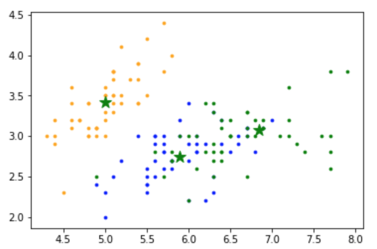

K-means from Scratch

from copy import deepcopy

# Number of clusters
K = 3
# Number of training data
n = X.shape[0]
# Number of features in the data
c = X.shape[1]

# Generate random centers, here we use sigma and mean to ensure it represent the whole data
mean = np.mean(X, axis = 0)
std = np.std(X, axis = 0)
centers = np.random.randn(K,c)*std + mean

centers_old = np.zeros(centers.shape) # to store old centers
centers_new = deepcopy(centers) # Store new centers

clusters = np.zeros(n)
distances = np.zeros((n,K))

error = np.linalg.norm(centers_new - centers_old)

# When, after an update, the estimate of that center stays the same, exit loop
while error != 0:
    # Measure the distance to every center
    for i in range(K):
        distances[:,i] = np.linalg.norm(X - centers_new[i], axis=1)
    # Assign all training data to closest center
    clusters = np.argmin(distances, axis = 1)
    
    centers_old = deepcopy(centers_new)
    # Calculate mean for every cluster and update the center
    for i in range(K):
        centers_new[i] = np.mean(X[clusters == i], axis=0)
    error = np.linalg.norm(centers_new - centers_old)
centers_new    
# array([[5.006     , 3.418     , 1.464     , 0.244     ],
#        [6.48787879, 2.96212121, 5.34242424, 1.87575758],
#        [5.82352941, 2.69705882, 4.05882353, 1.28823529]])

# Plot the data
colors=['orange', 'blue', 'green']
for i in range(n):
    plt.scatter(X[i, 0], X[i,1], s=7, color = colors[int(y[i])])
plt.scatter(centers_new[:,0], centers_new[:,1], marker='*', c='g', s=150)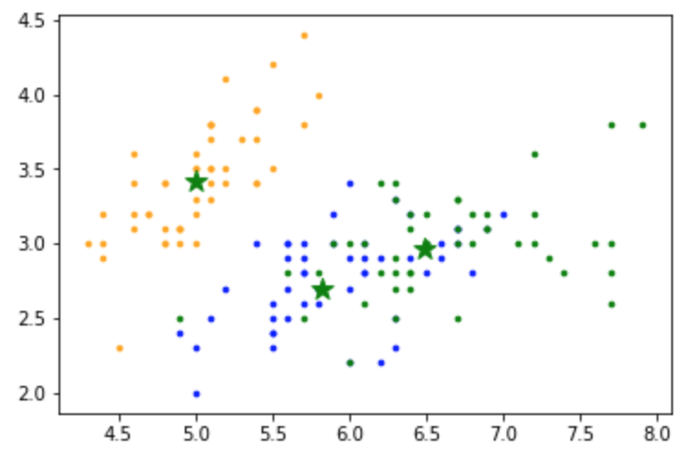

K-median

K-median is another clustering algorithm closely related to K-means. The practical difference between the two is as follows:

In K-means, centroids are determined by minimizing the sum of the squares of the distance between a centroid candidate and each of its examples.
In K-median, centroids are determined by minimizing the sum of the distance between a centroid candidate and each of its examples.

K-medians owes its use to robustness of the median as a statistic. The mean is a measurement that is highly vulnerable to outliers. Even just one drastic outlier can pull the value of the mean away from the majority of the data set, which can be a high concern when operating on very large data sets. The median, on the other hand, is a statistic incredibly resistant to outliers, for in order to deter the median away from the bulk of the information, it requires at least 50% of the data to be contaminated

K-medians uses the median as the statistic to determine the center of each cluster.

Note that the definitions of distance are also different:

K-means relies on the Euclidean distance from the centroid to an example. (In two dimensions, the Euclidean distance means using the Pythagorean theorem to calculate the hypotenuse.) For example, the K-means distance between $(2,2)$ and $(5,-2)$ would be:
\[\text{Euclidean Distance} = \sqrt{(2-5)^{2} + (2 - -2)^{2}} =5\]
K-median relies on the Manhattan distance from the centroid to an example. This distance is the sum of the absolute deltas in each dimension. For example, the K-median distance between $(2,2)$ and $(5,-2)$ would be:
\[\text{Manhattan Distance} = \lvert 2-5 \rvert + \lvert 2 - -2 \rvert = 7\]

Note that K-medians is also very sensitive to the initialization points of its K centers, each center having the tendency to remain roughly in the same cluster in which it is first placed.

Mini Batch K-Means

The Mini-batch K-Means is a variant of the K-Means algorithm which uses mini-batches to reduce the computation time, while still attempting to optimise the same objective function. Mini-batches are subsets of the input data, randomly sampled in each training iteration. These mini-batches drastically reduce the amount of computation required to converge to a local solution. In contrast to other algorithms that reduce the convergence time of K-means, mini-batch K-means produces results that are generally only slightly worse than the standard algorithm.

The algorithm iterates between two major steps, similar to vanilla K-means. In the first step, samples are drawn randomly from the dataset, to form a mini-batch. These are then assigned to the nearest centroid. In the second step, the centroids are updated. In contrast to k-means, this is done on a per-sample basis. For each sample in the mini-batch, the assigned centroid is updated by taking the streaming average of the sample and all previous samples assigned to that centroid. This has the effect of decreasing the rate of change for a centroid over time. These steps are performed until convergence or a predetermined number of iterations is reached.

Mini-batch K-Means converges faster than K-Means, but the quality of the results is reduced. In practice this difference in quality can be quite small.

For details, look here

REFERENCES

← → Top