on
16 mins to read.
A Complete Guide to K-Nearest-Neighbors with Applications in Python
Let’s first start by establishing some definitions and notations. We will use $x$ to denote a feature (aka. predictor, attribute) and $y$ to denote the target (aka. label, class) we are trying to predict.
K-NN falls in the supervised learning family of algorithms. Informally, this means that we are given a labelled dataset consiting of training observations $(x,y)$ and would like to capture the relationship between $x$ and $y$. More formally, our goal is to learn a function $h: X \Rightarrow Y$ so that given an unseen observation $x$, $h(x)$ can confidently predict the corresponding output y.
The K-NN classifier is also a non parametric, instance-based and a lazy learning algorithm.
Non-parametric means there is no assumption for underlying data distribution. In other words, the model structure determined from the dataset. This will be very helpful in practice where most of the real world datasets do not follow mathematical theoretical assumptions. it makes no explicit assumptions about the functional form of $h$, avoiding the dangers of mismodeling the underlying distribution of the data. For example, suppose our data is highly non-Gaussian but the learning model we choose assumes a Gaussian form. In that case, our algorithm would make extremely poor predictions.
Instance-based learning means that our algorithm doesn’t explicitly learn a model. Instead, it chooses to memorize the training instances which are subsequently used as “knowledge” for the prediction phase. Concretely, this means that only when a query to our database is made (i.e. when we ask it to predict a label given an input), will the algorithm use the training instances to spit out an answer.
Lazy algorithm means it doesn’t learn a discriminative function from the training data but memorizes the training dataset instead (there is no need for learning or training of the model and all of the data points used at the time of prediction. An eager learner has a model fitting or training step. A lazy learner does not have a training phase). For example, the logistic regression algorithm learns the model weights during training time. In contrast, there is no training time in K-NN algorithm. It does not need any training data points for model generation. All training data used in the testing phase. This makes training faster and testing phase slower and costlier. Costly testing phase means time and memory. In the worst case, K-NN needs more time to scan all data points and scanning all data points will require more memory for storing training data.
Lazy learners do less work in the training phase and more work in the testing phase to make a classification. Lazy learners are also known as instance-based learners because lazy learners store the training points or instances, and all learning is based on instances.
How does the K-NN algorithm work?
In K-NN, K is the number of nearest neighbors. The number of neighbors is the core deciding factor. K is generally an odd number in order to prevent a tie. When $K = 1$, then the algorithm is known as the nearest neighbor algorithm. This is the simplest case
In the classification setting, the K-nearest neighbor algorithm essentially boils down to forming a majority vote between the K most similar instances (K-nearest neighbors) to a given “unseen” observation. Similarity is defined according to a distance metric between two data points. A case is classified by a majority vote of its neighbors, with the case being assigned to the class most common amongst its K nearest neighbors measured by a distance function.
A popular choice is the Euclidean distance given by
\[d(x, x') = \sqrt{\left(x_1 - x'_1 \right)^2 + \left(x_2 - x'_2 \right)^2 + \dotsc + \left(x_n - x'_n \right)^2}\]but other measures can be more suitable for a given setting and include the Manhattan, Chebyshev, Minkowski et cetera..
It should also be noted that all three distance measures are only valid for continuous variables. In the instance of categorical variables the Hamming distance must be used. It also brings up the issue of standardization of the numerical variables between 0 and 1 when there is a mixture of numerical and categorical variables in the dataset.
More formally, given a positive integer K, an unseen observation $x$ and a similarity metric $d$, K-NN classifier performs the following two steps:
-
It runs through the whole dataset computing distance between $x$ and each training observation. We’ll call the ‘K points in the training data that are closest to x’ the set $\mathcal{A}$. Note that K is usually odd to prevent tie situations.
-
It then estimates the conditional probability for each class, that is, the fraction of points in $\mathcal{A}$ with that given class label. (Note $I(x)$ is the indicator function which evaluates to 1 when the argument x is true and 0 otherwise)
Finally, our input x gets assigned to the class with the largest probability.

How do you decide the number of neighbors in K-NN?
The number of neighbors (K) in K-NN is a hyperparameter that you need choose at the time of model building. You can think of K as a controlling variable for the prediction model. Choosing the optimal value for K is best done by first inspecting the data. Research has shown that no optimal number of neighbors suits all kind of data sets. In general, a large K value is more precise as it reduces the overall noise, is more resilient to outliers. Larger values of K will have smoother decision boundaries which means lower variance but increased bias, unlike a small value for K provides the most flexible fit, which will have low bias but high variance, but there is no guarantee.
- large K = not-flexible model = underfit = low variance & high bias
- small K = flexible model = overfit = high variance & low bias (for example, a k-NN model with K=1 will result in zero training error, typical for severe overfitting).
Cross-validation is another way to retrospectively determine a good K value by using an independent dataset to validate the K value. Historically, the optimal K for most datasets has been between 3-10. That produces much better results than 1NN.
Important thing to note in K-NN algorithm is the that the number of features and the number of classes both do not play a part in determining the value of K in K-NN algorithm. K-NN algorithm is an ad-hoc classifier used to classify test data based on distance metric. However, the value of K is non-parametric and a general rule of thumb in choosing the value of K is $K = \sqrt{n}$, where $n$ stands for the number of samples in the training dataset. Another tip is to try and keep the value of K odd, so that there is no tie between choosing a class .
Pros and Cons of this algorithm
Pros
-
It is simple to understand and easy to implement.
-
KNN is called Lazy Learner (Instance based learning). The training phase of K-nearest neighbor classification is much faster compared to other classification algorithms. There is no need to train a model for generalization
-
K-NN can be useful in case of nonlinear data.
-
It can be used with the regression problem. Output value for the object is computed by the average of K closest neighbors value, $f(x) = \frac{1}{K} \sum_{i=1}^{K} y_{i}$.
-
Since the KNN algorithm requires no training before making predictions, new data can be added seamlessly which will not impact the accuracy of the algorithm.
Cons
-
The testing phase of K-nearest neighbor classification is slower and costlier in terms of time and memory, which is impractical in industry settings. It requires large memory for storing the entire training dataset for prediction.
-
K-NN requires scaling of data because K-NN uses the Euclidean distance between two data points to find nearest neighbors. Euclidean distance is sensitive to magnitudes. The features with high magnitudes will weight more than features with low magnitudes.
-
K-NN can suffer from skewed class distributions. For example, if a certain class is very frequent in the training set, it will tend to dominate the majority voting of the new example (large number = more common). A simple and effective way to remedy skewed class distributions is by implementing weighed voting. The class of each of the K neighbors is multiplied by a weight proportional to the inverse of the distance from that point to the given test point. This ensures that nearer neighbors contribute more to the final vote than the more distant ones.
-
K-NN also not suitable for high dimensional data because there is little difference between the nearest and farthest neighbor.
-
K-NN performs better with a lower number of features than a large number of features. You can say that when the number of features increases, then, it requires more data. Increase in dimension also leads to the problem of overfitting. To avoid overfitting, the needed data will need to grow exponentially as you increase the number of dimensions. As the amount of dimension increases, the distance between various data points increases as well which can make predictions are much less reliable. This problem of higher dimension is known as the Curse of Dimensionality.
A Basic Example
We are given a training data set with n = 6 observations of $p = 2$ input variables $x_1$, $x_2$ and one (qualitative) output $y$, the color Red or Blue:
| i | $x_{1}$ | $x_{2}$ | y |
|---|---|---|---|
| 1 | -1 | 3 | Red |
| 2 | 2 | 1 | Blue |
| 3 | -2 | 2 | Red |
| 4 | -1 | 2 | Blue |
| 5 | -1 | 0 | Blue |
| 6 | 1 | 1 | Red |
and we are interested in predicting the output for $x^{test} = \begin{bmatrix}1 & 2 \end{bmatrix}^{T}$. For this purpose, we will explore two different k-NN classifiers, one using $k = 1$ and one using $k = 3$.
First, we compute the Euclidean distance $\lVert x_{i} - x^{test} \rVert$ between each training data point $x_{i}$ and the test data point $x^{test}$, and then sort them in descending order.
| i | $\lVert x_{i} - x^{test} \rVert$ | $y_{i}$ |
|---|---|---|
| 6 | $\sqrt{1}$ | Red |
| 2 | $\sqrt{2}$ | Blue |
| 4 | $\sqrt{4}$ | Blue |
| 1 | $\sqrt{5}$ | Red |
| 5 | $\sqrt{8}$ | Blue |
| 3 | $\sqrt{9}$ | Red |
Since the closest training data point to $x^{test}$ is the data point $i = 6$ (Red), it means that for k-NN with $k = 1$, we get the model $p\left(\text{Red}\,\,\, \mid \,\,\, x^{test} \right) = 1$ and $p\left(\text{Blue}\,\,\, \mid \,\,\,x^{test}\right) = 0$. This gives the prediction $\hat{y}^{test} = Red$.
Further, for $k = 3$, the 3 nearest neighbors are $i = 6$ (Red), $i = 2$ (Blue), and $i = 4$ (Blue), which gives the model $p\left(\text{Red}\,\,\, \mid \,\,\, x^{test}\right) = \frac{1}{3}$ and $p\left(\text{Blue}\,\,\, \mid \,\,\, x^{test}\right) = \frac{2}{3}$. The prediction, which also can be seen as a majority vote among those 3 training data points, thus becomes $\hat{y}^{test} = Blue$.
DATA: Iris Flower Dataset
# loading libraries
import numpy as np
from sklearn.cross_validation import train_test_split
import pandas as pd
from sklearn.datasets import load_iris

data = load_iris()
X = data['data']
y = data['target']
# split into train and test
X_train, X_test, y_train, y_test = train_test_split(X, y, test_size=0.33, random_state=42)
K-NN in Sci-kit Learn
# loading library
from sklearn.neighbors import KNeighborsClassifier
from sklearn.metrics import accuracy_score

# instantiate learning model (k = 3)
knn = KNeighborsClassifier(n_neighbors=3)

# fitting the model
knn.fit(X_train, y_train)

# predict the response
pred = knn.predict(X_test)

# evaluate accuracy

print('\nThe accuracy of the classifier is {}%'.format(accuracy_score(y_test, pred)*100))
#The accuracy of the classifier is 98.0%
k-fold Cross Validation for a fixed K
from sklearn.model_selection import cross_val_score
import numpy as np

#create a new KNN model
knn_cv = KNeighborsClassifier(n_neighbors=3)
#train model with cv of 5
cv_scores = cross_val_score(knn_cv, X, y, cv=10)
#print each cv score (accuracy) and average them
print(cv_scores)
# [1.         0.93333333 1.         0.93333333 0.86666667 1.
#  0.93333333 1.         1.         1.        ]
print('cv_scores mean:{}'.format(np.mean(cv_scores)))
# cv_scores mean:0.9666666666666666
k-fold Cross Validation and Grid Search
When building an initial K-NN model, we set the parameter n_neighbors to any number as a starting point with no real logic behind that choice. In order to find optimal nearest neighbors, we will specify a range of values for n_neighbors in order to see which value works best for our model.
from sklearn.model_selection import GridSearchCV
#create new a knn model
knn2 = KNeighborsClassifier()
#create a dictionary of all values we want to test for n_neighbors
param_grid = {'n_neighbors': np.arange(1, 25)}
#use gridsearch to test all values for n_neighbors
knn_gscv = GridSearchCV(knn2, param_grid, cv=5)
#fit model to data
knn_gscv.fit(X, y)

#check top performing n_neighbors value
print(knn_gscv.best_params_)
# {'n_neighbors': 6}
print(knn_gscv.best_score_)
# 0.98

plt.plot(knn_gscv.cv_results_['param_n_neighbors'].data, knn_gscv.cv_results_['mean_test_score'])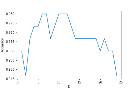
You do not need to use GridSearchCV package. It is easy to implement:
# search for an optimal value of K for KNN
# range of k we want to try
k_range = range(1, 31)
# empty list to store scores
k_scores = []

# 1. we will loop through reasonable values of k
for k in k_range:
    # 2. run KNeighborsClassifier with k neighbours
    knn = KNeighborsClassifier(n_neighbors=k)
    # 3. obtain cross_val_score for KNeighborsClassifier with k neighbours
    scores = cross_val_score(knn, X, y, cv=10, scoring='accuracy')
    # 4. append mean of scores for k neighbors to k_scores list
    k_scores.append(scores.mean())
print(k_scores)
K-NN from Scratch
from collections import Counter
from sklearn.metrics import accuracy_score

#In the case of KNN, which as discussed earlier, is a lazy algorithm, the training block reduces
#to just memorizing the training data.
def train(X_train, y_train):
    # do nothing
    return

def predict(X_train, y_train, x_test, k):
    # create list for distances and targets
    distances = []
    targets = []

    for i in range(len(X_train)):
        # first we compute the euclidean distance
        distance = np.sqrt(np.sum(np.square(x_test - X_train[i, :])))
        # add it to list of distances
        distances.append([distance, i])

    # sort the list
    distances = sorted(distances)
    # [[0.22360679774997896, 59],
    #  [0.30000000000000027, 70],
    #  [0.43588989435406783, 19],
    #  [0.5099019513592785, 53],
    #  ....
    #  [3.844476557348217, 97],
    #  [3.845776904605882, 46],
    #  [3.8961519477556315, 71],
    #  [3.9357337308308855, 52],
    #  [4.177319714841085, 47]]

    # make a list of the k neighbors' targets
    for i in range(k):
        index = distances[i][1]
        targets.append(y_train[index])

    # return most common target
    return Counter(targets).most_common(1)[0][0]

def kNearestNeighbor(X_train, y_train, X_test, k):
    # train on the input data
    train(X_train, y_train)

    predictions = []

    # loop over all observations
    for i in range(len(X_test)):
        predictions.append(predict(X_train, y_train, X_test[i, :], k))

    return np.asarray(predictions)

predictions = kNearestNeighbor(X_train, y_train, X_test, 7)

accuracy = accuracy_score(y_test, predictions)
print('\nThe accuracy of our classifier is {}%'.format(accuracy*100))
#The accuracy of our classifier is 98.0%
REFERENCES
- https://saravananthirumuruganathan.wordpress.com/2010/05/17/a-detailed-introduction-to-k-nearest-neighbor-knn-algorithm/
- https://kevinzakka.github.io/2016/07/13/k-nearest-neighbor/
- https://www.datacamp.com/community/tutorials/k-nearest-neighbor-classification-scikit-learn
- https://lyfat.wordpress.com/2012/05/22/euclidean-vs-chebyshev-vs-manhattan-distance/