Dimensions of matrices in an LSTM Cell

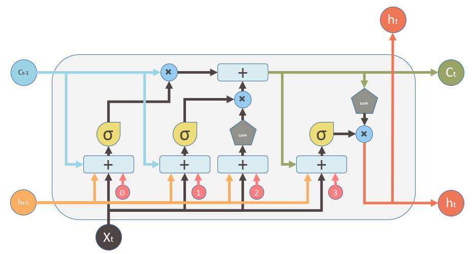
A general LSTM unit (not a cell! An LSTM cell consists of multiple units. Several LSTM cells form one LSTM layer.) can be shown as given below (source).

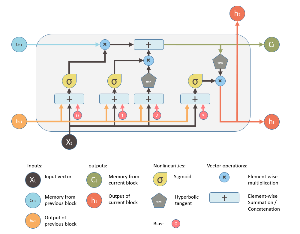
Equations below summarizes how to compute the unit’s long-term state, its short-term state, and its output at each time step for a single instance (the equations for a whole mini-batch are very similar).

1. Input gate: $ i_{t} = \sigma (W_{xi}^{T} \cdot X_{t} + W_{hi}^{T} \cdot h_{t-1} + b_{i})$

2. Forget gate: $ f_{t} = \sigma (W_{xf}^{T} \cdot X_{t} + W_{hf}^{T} \cdot h_{t-1} + b_{f})$

3. New Candidate: $ \widetilde{C_{t}} = tanh (W_{xc} \cdot X_{t} + W_{hc} \cdot h_{t-1} + b_{c})$

4. Cell State: $ C_{t} = f_{t}\circ C_{t-1} + i_{t} \circ \widetilde{C}_{t}$

5. Output gate: $ o_{t} = \sigma (W_{xo} \cdot X_{t} + W_{ho} \cdot h_{t-1} + b_{o})$

6. Hidden State: $ h_{t} = o_{t}\circ tanh(C_{t})$

• $W_{xi}$, $W_{xf}$, $W_{xc}$, $W_{xo}$ are the weight matrices of each of the three gates and block input for their connection to the input vector $X_{t}$.
• $W_{hi}$, $W_{hf}$, $W_{hc}$, $W_{ho}$ are the weight matrices of each of the three gates and block input for their connection to the previous short-term state $h_{t-1}$.
• $b_{i}$, $b_{f}$, $b_{c}$ and $b_{o}$ are the bias terms for each of the three gates and block input .
• $\sigma$ is an element-wise sigmoid activation function of the neurons, and $tanh$ is an element-wise hyperbolic tangent activation function of the neurons
• $\circ$ represents the Hadamard product (elementwise product).

NOTE: Sometimes, $h_t$ is called as the outgoing state and $c_t$ is called as the internal cell state.

source: https://stackoverflow.com/a/53760729

Just like for feedforward neural networks, we can compute all these in one shot for a whole mini-batch by placing all the inputs at time step $t$ in an input matrix $X_{t}$. If we write down the equations for all instances in a mini-batch, we will have:

1. Input gate: $ i_{t} = \sigma (X_{t}\cdot W_{xi} + h_{t-1} \cdot W_{hi} + b_{i})$

2. Forget gate: $ f_{t} = \sigma (X_{t} \cdot W_{xf} + h_{t-1} \cdot W_{hf} + b_{f})$

3. New Candidate: $ \widetilde{C_{t}} = tanh (X_{t} \cdot W_{xc} + h_{t-1} \cdot W_{hc} + b_{c})$

4. Cell State: $ C_{t} = f_{t}\circ C_{t-1} + i_{t} \circ \widetilde{C}_{t}$

5. Output gate: $ o_{t} = \sigma (X_{t} \cdot W_{xo} + h_{t-1} \cdot W_{ho} + b_{o})$

6. Hidden State: $ h_{t} = o_{t}\circ tanh(C_{t})$

We can concatenate the weight matrices for $X_{t}$ and $h_{t-1}$ horizontally, we can rewrite the equations above as the following:

1. Input gate: $ i_{t} = \sigma ( [X_{t} h_{t-1}] \cdot W_{i} + b_{i})$

2. Forget gate: $ f_{t} = \sigma ([X_{t} h_{t-1}] \cdot W_{f} + b_{f})$

3. New Candidate: $ \widetilde{C_{t}} = tanh ( [X_{t} h_{t-1}] \cdot W_{c} + b_{c})$

4. Cell State: $ C_{t} = f_{t}\circ C_{t-1} + i_{t} \circ \widetilde{C}_{t}$

5. Output gate: $ o_{t} = \sigma ([X_{t} h_{t-1}] \cdot W_{o}+ b_{o})$

6. Hidden State: $ h_{t} = o_{t}\circ tanh(C_{t})$

Tensorflow Dimensions

In Tensorflow, LSTM variables are defined in LSTMCell.build method. The source code can be found in rnn_cell_impl.py:

self._kernel = self.add_variable(
    _WEIGHTS_VARIABLE_NAME,
    shape=[input_depth + h_depth, 4 * self._num_units],
    initializer=self._initializer,
    partitioner=maybe_partitioner)
self._bias = self.add_variable(
    _BIAS_VARIABLE_NAME,
    shape=[4 * self._num_units],
    initializer=init_ops.zeros_initializer(dtype=self.dtype))

As one can see easily, there’s just one [input_depth + h_depth, 4 * self._num_units] shaped weight matrix and [4 * self._num_units] shaped bias vector, not 8 different matrices for weights and 4 different vectors for biases, and all of them are multiplied simultaneously in a batch.

The gates are defined this way:

# i = input_gate, j = new_input, f = forget_gate, o = output_gate
i, j, f, o = array_ops.split(value=gate_inputs, num_or_size_splits=4, axis=one)

Considering that we have a data, shape of [batch_size, time_steps, number_features], $X_{t}$ is the input of time-step $t$ which is an array with the shape of [batch_size, number_features], $h_{t-1}$ is the hidden state of previous time-step which is an array with the shape of [batch_size, number_units], and $C_{t-1}$ is the cell state of previous time-step, which is an array with the shape of [batch_size, num_units]. In that case, Tensorflow will concatenate inputs ($X_{t}$) and hidden state ($h_{t-1}$) by column and multiple it with kernel (weight) matrix that we mentioned previously. For more info, look at here.

Each of the $W_{xi}$, $W_{xf}$, $W_{xc}$ and $W_{xo}$, is an array with the shape of [number_features, number_units] and, similarly, each of the $W_{hi}$, $W_{hf}$, $W_{hc}$ and $W_{ho}$ is an array with the shape of [number_units, num_units]. If we first concatenate each gate weight matrices, corresponding to input and hidden state, vertically, we will have separate $W_{i}$, $W_{c}$, $W_{f}$ and $W_{o}$ matrices, which each will have the shape of [number_features + number_units, number_units]. Then, if we concatenate $W_{i}$, $W_{c}$, $W_{f}$ and $W_{o}$ matrices horizontally, we will have kernel (weights) matrix, given by Tensorflow, which has shape [number_features + number_units, 4 * number_units].

NOTE: Tensorflow uses the letter j to denote new input (candidate), we use the letter c.

Mathematical Representation

Let’s denote $B$ as batch size, $F$ as number of features and $U$ as number of units in an LSTM cell, therefore, the dimensions will be computed as follows:

$X_{t} \in \mathbb{R}^{B \times F}$

$h_{t-1} \in \mathbb{R}^{B \times U}$

$h_{t} \in \mathbb{R}^{B \times U}$

$C_{t-1} \in \mathbb{R}^{B \times U}$

$W_{xi} \in \mathbb{R}^{F \times U}$

$W_{xf} \in \mathbb{R}^{F \times U}$

$W_{xc} \in \mathbb{R}^{F \times U}$

$W_{xo} \in \mathbb{R}^{F \times U}$

$W_{hi} \in \mathbb{R}^{U \times U}$

$W_{hf} \in \mathbb{R}^{U \times U}$

$W_{hc} \in \mathbb{R}^{U \times U}$

$W_{ho} \in \mathbb{R}^{U \times U}$

$W_{i} \in \mathbb{R}^{F+U \times U}$

$W_{c} \in \mathbb{R}^{F+U \times U}$

$W_{f} \in \mathbb{R}^{F+U \times U}$

$W_{o} \in \mathbb{R}^{F+U \times U}$

$b_{i} \in \mathbb{R}^{U}$

$b_{c} \in \mathbb{R}^{U}$

$b_{f} \in \mathbb{R}^{U}$

$b_{o} \in \mathbb{R}^{U}$

$i_{t} \in \mathbb{R}^{B \times U}$

$f_{t} \in \mathbb{R}^{B \times U}$

$C_{t} \in \mathbb{R}^{B \times U}$

$h_{t} \in \mathbb{R}^{B \times U}$

$o_{t} \in \mathbb{R}^{B \times U}$

NOTE: Batch size can be $1$. In that case, $B=1$.

LSTM with Peephole Connections

In a basic LSTM cell, the gate controllers can look only at the input $X_{t}$, and the previous short-term state $h_{t-1}$. It may be a good idea to give them a bit more context by letting them peek at the long-term state as well. This LSTM variant with extra connections called peephole connections which lead from the cells to the gates: the previous long-term state $C_{t-1}$ is added as an input to the controllers of the forget gate and input gate, and the current long-term state $C_{t}$ is added to the controller of the output gate.

Based on the information above, if we write down the equations for all instances in a mini-batch, we will have:

1. Input gate: $ i_{t} = \sigma (X_{t} \cdot W_{xi} + h_{t-1} \cdot W_{hi} + C_{t-1}\circ W_{ci} + b_{i})$

2. Forget gate: $ f_{t} = \sigma (X_{t} \cdot W_{xf} + h_{t-1} \cdot W_{hf} + C_{t-1}\circ W_{cf} + b_{f})$

3. New Candidate: $ \widetilde{C_{t}} = tanh (X_{t} \cdot W_{xc} + h_{t-1} \cdot W_{hc}+ b_{c})$

4. Cell State: $ C_{t} = f_{t}\circ C_{t-1} + i_{t} \circ \widetilde{C}_{t}$

5. Output gate: $ o_{t} = \sigma (X_{t} \cdot W_{xo} + h_{t-1} \cdot W_{ho} + C_{t}\circ W_{co} + b_{o})$

6. Hidden State: $ h_{t} = o_{t}\circ tanh(C_{t})$

Here, $\circ$ represents the Hadamard product (elementwise product).

Tensorflow implementation is given as follows:

      # Diagonal connections
      if self._use_peepholes:
        w_f_diag = vs.get_variable(
            "W_F_diag", shape=[self._num_units], dtype=dtype)
        w_i_diag = vs.get_variable(
            "W_I_diag", shape=[self._num_units], dtype=dtype)
        w_o_diag = vs.get_variable(
            "W_O_diag", shape=[self._num_units], dtype=dtype)
      if self._use_peepholes:
        c = (sigmoid(f + 1 + w_f_diag * c_prev) * c_prev +
             sigmoid(i + w_i_diag * c_prev) * tanh(j))
      else:
        c = (sigmoid(f + 1) * c_prev + sigmoid(i) * tanh(j))

As one can easily see that, the weights for peephole connections are one dimensional array, shape of [num_units].

Backward Pass

Backward pass of LSTM is computed as follows and all those equations are provided in this paper:

Here $\Delta_{t}$ is the vector of deltas passed down from the layer above. If $L$ is the loss function it formally corresponds to $\frac{\partial L}{\partial y_{t}}$ but not including the recurrent dependencies.

The final updates to the internal parameters is computed as:

where

$\circ$ represents Hadamard product. $\cdot$ is inner product. $\otimes$ is the outer product. $\Delta_{t}$ is differential difference between predicted output and actual output.

After computing the deltas, we can update the parameters based on the SGD update function:

where $\alpha$ is the step size (sometimes called the learning rate in machine learning).

NOTE: If you are cuyrious how LSTM netwoirks prevent vanishing gradients problem, click here.

What is the number of units in an LSTM cell?

It can be hard to understand what number of units in an LSTM cell stands for. Most LSTM diagrams just show the hidden cells but never the units of those cells. The image below from this source explains it very well. num_units can be interpreted as the analogy of hidden layer from the feed forward neural network. The number of units in an LSTM cell can be thought of number of neurons in a hidden layer. It is a direct representation of the learning capacity of a neural network.

https://stackoverflow.com/questions/37901047/what-is-num-units-in-tensorflow-basiclstmcell#:~:text=Tensorflow’s%20num_units%20is%20the%20size,memory%20units%20in%20the%20cell.

NOTES

Dot product can be confusing so I am hoping that these definitions might help. The hypothesis of each data point can be vectorized using following formula:

which is nothing but a linear regression equation for one instance in the data. Here, $x_{0}^{(i)} = 1$ because of the bias (intercept) in the equation.

In order to achieve the hypothesis for all the instances, we use the following array dot product:

Here, we assume that we have $m$ observations and $n$ input variables (features).