Written by MMA
on February 07, 2019
16 mins to read.

Backpropagation Through Time for Recurrent Neural Network

The dynamical system is defined by:

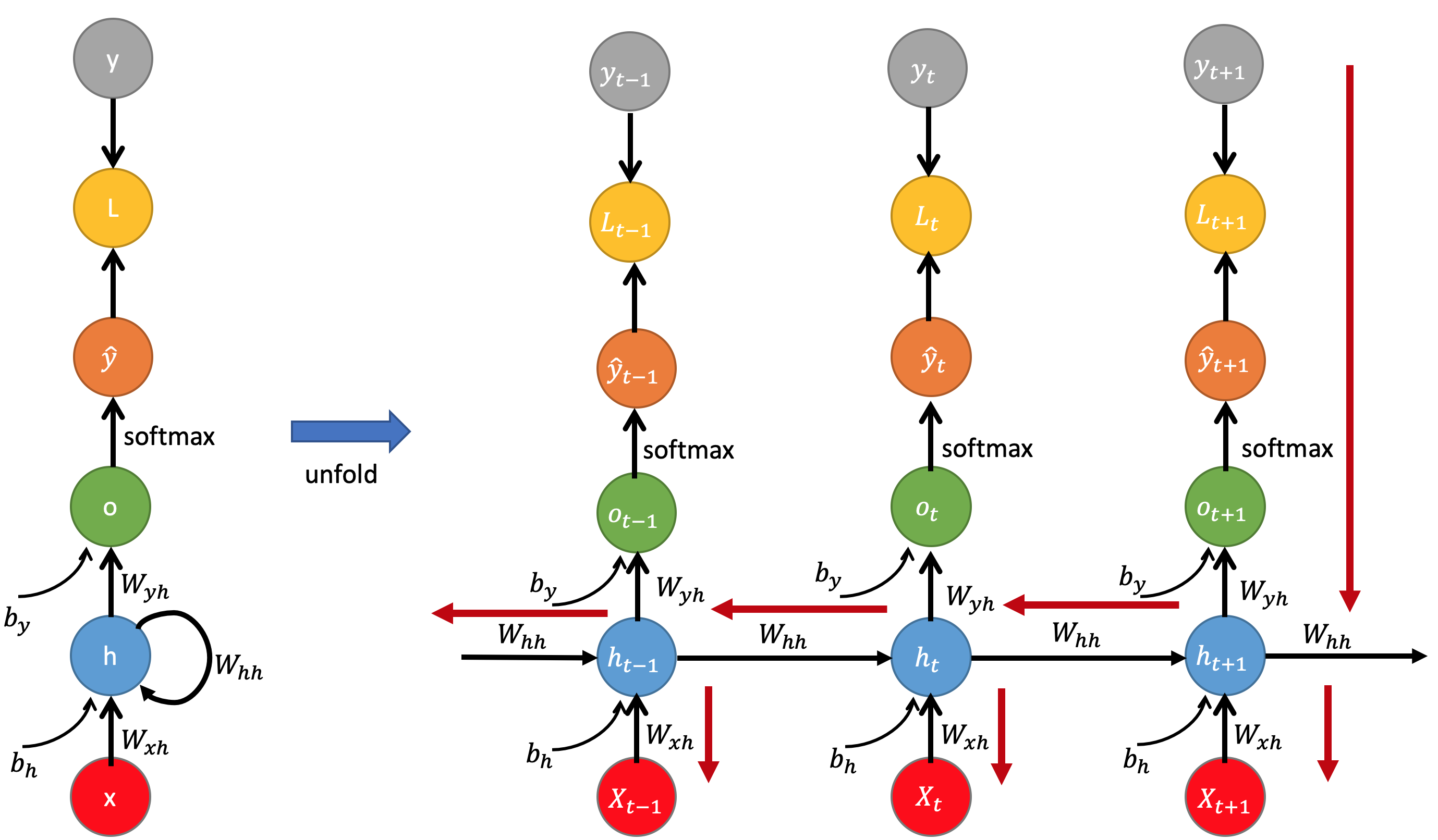
\[\begin{split} h_{t} & = f_{h} (X_{t}, h_{t-1})\\ \hat{y}_{t} &= f_{o}(h_{t}) \end{split}\]

A conventional RNN is constructed by defining the transition function and the output function for a single instance:

\[\begin{split} h_{t} & = f_{h} (X_{t}, h_{t-1}) = \phi_{h}(W_{xh}^{T} \cdot X_{t} + W_{hh}^{T}\cdot h_{t-1} +b_{h})\\ \hat{y}_{t} &= f_{o}(h_{t}) = \phi_{o}(W_{yh}^{T}\cdot h_{t} + b_{y}) \end{split}\]

where $W_{xh}$, $W_{hh}$ and $W_{yh}$ are weight matrices for the input, reccurent connections, and the output, respectively and $\phi_{h}$ and $\phi_{o}$ are element-wise nonlinear functions. It is usual to use a saturating nonlinear function such as logistic sigmoid function or a hyperbolic tangent function for $\phi_{h}$. $\phi_{o}$ is generally softmax activation for classification problem.

NOTE: Reusing same weight matrix every time step! $W$ is shared across time - reduces the number of parameters!

Just like for feedforward neural networks, we can compute a recurrent layer’s output in one shot for a whole mini-batch by placing all the inputs at time step $t$ in an input matrix $X_{t}$:

\[\begin{split} h_{t} & = tanh(X_{t}\cdot W_{xh} + h_{t-1}\cdot W_{hh} + b_{h})\\ &= \phi_{h}( [X_{t} h_{t-1}] \cdot W + b_{h})\\ o_{t} &= h_{t}\cdot W_{yh} + b_{y}\\ \hat{y}_{t} &= softmax(o_{t}) \end{split}\]

The weight matrices $W_{xh}$ and $W_{yh}$ are often concatenated vertically into a single weight matrix $W$ of shape $(n_{inputs} + n_{neurons}) \times n_{neurons}$.
The notation $[X_{t} h_{t-1}]$ represents the horizontal concatenation of the matrices $X_{t}$ and $h_{t-1}$, shape of $m \times (n_{inputs} + n_{neurons})$

Let’s denote $m$ as the number of instances in the mini-batch, $n_{neurons}$ as the number of neurons, and $n_{inputs}$ as the number of input features.

$X_{t}$ is an $m \times n_{inputs}$ matrix containing the inputs for all instances.
$h_{t-1}$ is an $m \times n_{neurons}$ matrix containing the hidden state of the previous time-step for all instances.
$W_{xh}$ is an $n_{inputs} \times n_{neurons}$ matrix containing the connection weights between input and the hidden layer.
$W_{hh}$ is an $n_{neurons} \times n_{neurons}$ matrix containing the connection weights between two hidden layers.
$W_{yh}$ is an $n_{neurons} \times n_{neurons}$ matrix containing the connection weights between the hidden layer and the output.
$b_{h}$ is a vector of size $n_{neurons}$ containing each neuron’s bias term.
$b_{y}$ is a vector of size $n_{neurons}$ containing each output’s bias term.
$y_{t}$ is an $m \times n_{neurons}$ matrix containing the layer’s outputs at time step $t$ for each instance in the mini-batch

NOTE: At the first time step, $t = 0$, there are no previous outputs, so they are typically assumed to be all zeros.

Backpropagation Through Time

In order to do backpropagation through time to train an RNN, we need to compute the loss function first:

\[\begin{split} L (\hat{y}, y) & = \sum_{t = 1}^{T} L_{t}(\hat{y}_{t}, y_{t}) \\ & = - \sum_{t}^{T} y_{t} \log \hat{y}_{t} \\ & = -\sum_{t = 1}^{T}y_{t} log \left[softmax(o_{t}) \right] \end{split}\]

Note that the weight $W_{yh}$ is shared across all the time sequence. Therefore, we can differentiate to it at the each time step and sum all together:

\[\begin{split} \frac{\partial L}{\partial W_{yh}} &= \sum_{t}^{T} \frac{\partial L_{t}}{\partial W_{yh}} \\ &= \sum_{t}^{T} \frac{\partial L_{t}}{\partial \hat{y}_{t}} \frac{\partial \hat{y}_{t}}{\partial o_{t}} \frac{\partial o_{t}}{\partial W_{yh}}\\ &=\sum_{t}^{T} (\hat{y}_{t} - y_{t}) \otimes h_{t} \end{split}\]

where derivative of Loss Function w.r.t. softmax function is proved here and $\frac{\partial o_{t}}{\partial W_{yh}} = h_{t}$ since $o_{t} = h_{t}\cdot W_{yh} + b_{y}$ and $\otimes$ is the outer product of two vectors.

Similarly, we can get the gradient w.r.t. bias $b_{y}$:

\[\begin{split} \frac{\partial L}{\partial b_{y}} &= \sum_{t}^{T} \frac{\partial L_{t}}{\partial \hat{y}_{t}} \frac{\partial \hat{y}_{t}}{\partial o_{t}} \frac{\partial o_{t}}{\partial b_{y}}\\ &=\sum_{t}^{T} (\hat{y}_{t} - y_{t}) \end{split}\]

Further, let’s use $L_{t+1}$ to denote the output of the time-step $t+1$, $L_{t+1} = -y_{t+1} log \hat{y}_{t+1}$.

Now, let’s go throught the details to derive the gradient with respect to $W_{hh}$, considering at the time step $t \rightarrow t+1$ (from time-step $t$ to $t+1$).

\[\frac{\partial L_{t+1}}{\partial W_{hh}} = \frac{\partial L_{t+1}}{\partial \hat{y}_{t+1}} \frac{\partial \hat{y}_{t+1}}{\partial h_{t+1}} \frac{\partial h_{t+1}}{\partial W_{hh}}\]

where we consider only one time-step ($t \rightarrow t+1$). But, the hidden state $h_{t+1}$ partially depends also on $h_{t}$ according to the recursive formulation ($h_{t} = tanh(W_{xh}^{T} \cdot X_{t} + W_{hh}^{T}\cdot h_{t-1} +b_{h})$). Thus, at the time-step $t-1 \rightarrow t$, we can further get the partial derivative with respect to $W_{hh}$ as the following:

\[\frac{\partial L_{t+1}}{\partial W_{hh}} = \frac{\partial L_{t+1}}{\partial \hat{y}_{t+1}} \frac{\partial \hat{y}_{t+1}}{\partial h_{t+1}}\frac{\partial h_{t+1}}{\partial h_{t}} \frac{\partial h_{t}}{\partial W_{hh}}\]

Thus, at the time-step $t+1$, we can compute the gradient and further use backpropagation through time from $t+1$ to $1$ to compute the overall gradient with respect to $W_{hh}$:

\[\frac{\partial L_{t+1}}{\partial W_{hh}} = \sum_{k=1}^{t+1} \frac{\partial L_{t+1}}{\partial \hat{y}_{t+1}} \frac{\partial \hat{y}_{t+1}}{\partial h_{t+1}}\frac{\partial h_{t+1}}{\partial h_{k}} \frac{\partial h_{k}}{\partial W_{hh}}\]

Note that $\frac{\partial h_{t+1}}{\partial h_{k}}$ is a chain rule in itself! For example, $\frac{\partial h_{3}}{\partial h_{1}} = \frac{\partial h_{3}}{\partial h_{2}}\frac{\partial h_{2}}{\partial h_{1}}$. Also note that because we are taking the derivative of a vector function with respect to a vector, the result is a matrix (called the Jacobian matrix) whose elements are all the pointwise derivatives. We can rewrite the above gradient:

\[\frac{\partial L_{t+1}}{\partial W_{hh}} = \sum_{k=1}^{t+1} \frac{\partial L_{t+1}}{\partial \hat{y}_{t+1}} \frac{\partial \hat{y}_{t+1}}{\partial h_{t+1}} \left( \prod_{j = k} ^{t} \frac{\partial h_{j+1}}{\partial h_{j}} \right) \frac{\partial h_{k}}{\partial W_{hh}}\]

where

\[\prod^{t}_{j=k} \frac{\partial h_{j+1}}{\partial h_{j}} = \frac{\partial h_{t+1}}{\partial h_k} = \frac{\partial h_{t+1}}{\partial h_{t}}\frac{\partial h_{t}}{\partial h_{t-1}}...\frac{\partial h_{k+1}}{\partial h_k}\]

NOTE: It turns out that the 2-norm, which you can think of it as an absolute value, of the above Jacobian matrix has an upper bound of 1. This makes intuitive sense because our tanh (or sigmoid) activation function maps all values into a range between -1 and 1, and the derivative is bounded by 1 (1/4 in the case of sigmoid) as well.

Let’s continue…

Aggregate the gradients with respect to $W_{hh}$ over the whole time-steps with backpropagation, we can finally yield the following gradient with respect to $W_{hh}$:

\[\frac{\partial L}{\partial W_{hh}} = \sum_{t}^{T} \sum_{k=1}^{t+1} \frac{\partial L_{t+1}}{\partial \hat{y}_{t+1}} \frac{\partial \hat{y}_{t+1}}{\partial h_{t+1}} \frac{\partial h_{t+1}}{\partial h_{k}}\frac{\partial h_{k}}{\partial W_{hh}}\]

Now, let’s work on to derive the gradient with respect to $W_{xh}$. Similarly, we consider the time-step $t+1$ (which gets only contribution from $X_{t+1}$) and calculate the gradients with respect to $W_{xh}$ as follows:

\[\frac{\partial L_{t+1}}{\partial W_{xh}} = \frac{\partial L_{t+1}}{\partial \hat{y}_{t+1}} \frac{\partial \hat{y}_{t+1}}{\partial h_{t+1}}\frac{\partial h_{t+1}}{\partial W_{xh}}\]

Because $h_{t}$ and $X_{t+1}$ both make contribution to $h_{t+1}$, we need to backpropagate to $h_{t}$ as well.

If we consider the contribution from the time-step, we can further get:

\[\frac{\partial L_{t+1}}{\partial W_{xh}} = \frac{\partial L_{t+1}}{\partial \hat{y}_{t+1}} \frac{\partial \hat{y}_{t+1}}{\partial h_{t+1}}\frac{\partial h_{t+1}}{\partial W_{xh}} + \frac{\partial L_{t+1}}{\partial \hat{y}_{t+1}} \frac{\partial \hat{y}_{t+1}}{\partial h_{t+1}}\frac{\partial h_{t+1}}{\partial h_{t}} \frac{\partial h_{t}}{\partial W_{xh}}\]

Thus, summing up all the contributions from $t+1$ to $1$ via Backpropagation, we can yield the gradient at the time-step $t+1$:

\[\frac{\partial L_{t+1}}{\partial W_{xh}} = \sum_{k=1}^{t+1} \frac{\partial L_{t+1}}{\partial \hat{y}_{t+1}} \frac{\partial \hat{y}_{t+1}}{\partial h_{t+1}}\frac{\partial h_{t+1}}{\partial h_{k}} \frac{\partial h_{k}}{\partial W_{xh}}\]

Further, we can take the derivative with respect to $W_{xh}$ over the whole sequence as :

\[\frac{\partial L} {\partial W_{xh}} = \sum_{t}^{T} \sum_{k=1}^{t+1} \frac{\partial L_{t+1}}{\partial \hat{y}_{t+1}} \frac{\partial \hat{y}_{t+1}}{\partial h_{t+1}} \frac{\partial h_{t+1}}{\partial h_{k}} \frac{\partial h_{k}}{\partial W_{xh}}\]

Do not forget that $\frac{\partial h_{t+1}}{\partial h_{k}}$ is a chain rule in itself, again!

Vanishing/Exploding Gradients with vanilla RNNs

There are two factors that affect the magnitude of gradients - the weights and the activation functions (or more precisely, their derivatives) that the gradient passes through. In vanilla RNNs, vanishing/exploding gradient comes from the repeated application of the recurrent connections. More explicitly, they happen because of recursive derivative we need to compute $\frac{\partial h_{t+1}}{\partial h_k}$:

Now let us look at a single one of these terms by taking the derivative of $h_{j+1}$ with respect to $h_{j}$ where diag turns a vector into a diagonal matrix because this recursive partial derivative is a Jacobian matrix:

\[\frac{\partial h_{j+1}}{\partial h_{j}} = diag(\phi_{h}^{\prime}(W_{xh}^{T} \cdot X_{j+1} + W_{hh}^{T}\cdot h_{j} +b_{h})W_{hh}\]

Thus, if we want to backpropagate through $t-k$ timesteps, this gradient will be:

\[\prod^{t}_{j=k} \frac{\partial h_{j+1}}{\partial h_{j}} = \prod^{t}_{j=k} diag(\phi_{h}^{\prime}(W_{xh}^{T} \cdot X_{j+1} + W_{hh}^{T}\cdot h_{j} +b_{h})W_{hh}\]

If we perform eigendecomposition on the Jacobian matrix $\frac{\partial h_{j+1}}{\partial h_{j}}$, we get the eigenvalues $\lambda_{1}, \lambda_{2}, \cdots, \lambda_{n}$ where $\lvert\lambda_{1}\rvert \gt \lvert\lambda_{2}\rvert \gt\cdots \gt \lvert\lambda_{n}\rvert$ and the corresponding eigenvectors $v_{1}, v_{1},\cdots,v_{n}$.

Any change on the hidden state $\Delta h_{j+1}$ in the direction of a vector $v_{i}$ has the effect of multiplying the change with the eigenvalue associated with this eigenvector i.e $\lambda_{i}\Delta h_{j+1}$.

The product of these Jacobians implies that subsequent time steps, will result in scaling the change with a factor equivalent to $\lambda_{i}^{t}$, where $\lambda_{i}^{t}$ represents the $i$-th eigenvalue raised to the power of the current time step $t$.

Looking at the sequence $\lambda_{i}^{1}\Delta h_{1}, \lambda_{i}^{2}\Delta h_{2}, \dots, \lambda_{n}^{1}\Delta h_{n}$, it is easy to see that the factor $\lambda_{i}^{t}$ will end up dominating the $\Delta h_{t}$’s because this term grows exponentially fast as $t$ goes to infinity.

This means that if the largest eigenvalue $\lambda_{1} <1$ then the gradient will vanish while if the value of $\lambda_{1} > 1$, the gradient explodes.

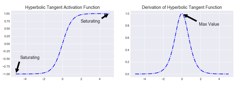
As also shown in this paper, if the dominant eigenvalue of the matrix $W_{hh}$ is greater than 1, the gradient explodes. If it is less than 1, the gradient vanishes. The fact that this equation leads to either vanishing or exploding gradients should make intuitive sense. Note that the values of $\phi_{h}^{\prime}$ will always be less than 1. Because in vanilla RNN, the activation function $\phi_{h}$ is used to be hyperbolic tangent whose derivative is at most $1.0$. So if the magnitude of the values of $W_{hh}$ are too small, then inevitably the derivative will go to 0. The repeated multiplications of values less than one would overpower the repeated multiplications of $W_{hh}$. On the contrary, make $W_{hh}$ too big and the derivative will go to infinity since the exponentiation of $W_{hh}$ will overpower the repeated multiplication of the values less than 1.

Vanishing gradients aren’t exclusive to RNNs. They also happen in deep Feedforward Neural Networks. It’s just that RNNs tend to be very deep, which makes the problem a lot more common.

These problems ultimately shows that if the gradient vanishes, it means that the earlier hidden states have no real effect on the later hidden states, meaning no long term dependencies are learned!

Fortunately, there are a few ways to come over the vanishing gradient problem. Proper initialization of the weight matrices can reduce the effect of vanishing gradients. So can regularization. A more preferred solution is to use ReLU activation function instead of hyperbolic tangent or sigmoid activation functions. The ReLU derivative is a constant of either 0 or 1, so it isn’t as likely to suffer from vanishing gradients. An even more popular solution is to use Long Short-Term Memory (LSTM) or Gated Recurrent Unit (GRU) architectures.

Additional Explanation

Let’s take the norms of these Jacobians:

\[\left\Vert \frac{\partial h_{j+1}}{\partial h_{j}} \right\Vert \leq \left\Vert W_{hh} \right\Vert \left\Vert diag(\phi_{h}^{\prime}(W_{xh}^{T} \cdot X_{j+1} + W_{hh}^{T}\cdot h_{j} +b_{h}) \right\Vert\]

In this equation, we set $\gamma_{W}$, the largest eigenvalue associated with $\left\Vert W_{hh} \right\Vert$ as its upper bound, while $\gamma_{h}$ largest eigenvalue associated with $\left\Vert diag(\phi_{h}^{\prime}(W_{xh}^{T} \cdot X_{j+1} + W_{hh}^{T}\cdot h_{j} +b_{h}) \right\Vert$ as its corresponding upper-bound.

Depending on the chosen activation function $\phi_{h}$, the derivative $\phi_{h}^{\prime}$ will be upper bounded by different values. For hyperbolic tangent function, we have $\gamma_{h} = 1$ while for sigmoid function, we have $\gamma_{h} = 0.25$. Thus, the chosen upper bounds $\gamma_{W}$ and $\gamma_{h}$ end up being a constant term resulting from their product:

The gradient $\frac{\partial h_{t+1}}{\partial h_k}$ is a product of Jacobian matrices that are multiplied many times, $t-k$ times in our case:

\[\left\Vert \frac{\partial h_{t+1}}{\partial h_k} \right\Vert = \left\Vert \prod^{t}_{j=k} \frac{\partial h_{j+1}}{\partial h_{j}} \right\Vert \leq (\gamma_{W} \gamma_{h})^{t-k}\]

This can become very small or very large quickly, and the locality assumption of gradient descent breaks down as the sequence gets longer (i.e the distance between $t$ and $k$ increases). Then the value of $\gamma$ will determine if the gradient either gets very large (explodes) or gets very small (vanishes).

Since $\gamma$ is associated with the leading eigenvalues of $ \frac{\partial h_{j+1}}{\partial h_{j}}$, the recursive product of $t-k$ Jacobian matrices makes it possible to influence the overall gradient in such a way that for $\gamma < 1$ the gradient tends to vanish while for $\gamma > 1$ the gradient tends to explode.

Vanishing/Exploding Gradients with LSTMs

As can be seen easily above, the biggest problem with causing gradients to vanish is the multiplication of recursive derivatives. One of the approaches that was proposed to overcome this issue is to use gated structures such as Long Short-Term Memory Networks.

In the original LSTM formulation, the value of $C_{t}$ depends on the previous value of cell state and an update term weighted by the input gate (pp. 7):

which we can re-write it in our terms as:

\[C_{t} = C_{t-1} + i_{t} \circ \widetilde{C}_{t}\]

The original motivation behind this LSTM was to make this recursive derivative have a constant value, which was equal to 1 because of the truncated BPTT algorithm. In other words, the gradient calculation was truncated so as not to flow back to the input or candidate gates. If this is the case, then our gradients would neither explode or vanish. However, this formulation doesn’t work well because the cell state tends to grow uncontrollably. In order to prevent this unbounded growth, a forget gate was added to scale the previous cell state, leading to the more modern formulation (Appendix A):

which we can re-write it in our terms as:

\[C_{t} = f_{t}\circ C_{t-1} + i_{t} \circ \widetilde{C}_{t}\]

However, there are so many documents out there online, that claim that the reason of LSTM solving this vanishing gradient problem is that under this update rule the recursive derivative is equal to 1 in the case of original LSTM or $f$ (forget gate) in the case of modern LSTM. However, $f_{t}$, $i_{t}$ and $\widetilde{C_{t}}$ are all functions of $C_{t}$ and so we have to take them into consideration when calculating the derivation of $C_{t}$ with respect to $C_{t-1}$ .

NOTE: In the case of the forget gate LSTM, the recursive derivative will still be a produce of many terms between 0 and 1 (the forget gates at each time step), however in practice this is not as much of a problem compared to the case of RNNs. One thing to remember is that our network has direct control over what the values of $f$ will be. If it needs to remember something, it can easily set the value of $f$ to be high (lets say around 0.95). These values thus tend to shrink at a much slower rate than when compared to the derivative values of hyperbolic tangent function, which later on during the training processes, are likely to be saturated and thus have a value close to 0.

Therefore, let’s find the full derivative $\frac{\partial C_{t}}{\partial C_{t-1}}$. Remember that $C_{t}$ is a function of $f_{t}$ (the forget gate), $i_{t}$ (input gate) and $\widetilde{C_{t}}$ (candidate input), each of these being a function of $C_{t-1}$ (since they are all functions of $h_{t-1}$). Via the multivariate chain rule we get:

\[\frac{\partial C_{t}}{\partial C_{t-1}} = \frac{\partial C_{t}}{\partial f_{t}} \frac{\partial f_{t}}{\partial h_{t-1}} \frac{\partial h_{t-1}}{\partial C_{t-1}} + \frac{\partial C_{t}}{\partial i_{t}} \frac{\partial i_{t}}{\partial h_{t-1}} \frac{\partial h_{t-1}}{\partial C_{t-1}} + \frac{\partial C_{t}}{\partial \widetilde{C}_{t}} \frac{\partial \widetilde{C}_{t}}{\partial h_{t-1}} \frac{\partial h_{t-1}}{\partial C_{t-1}} + \frac{\partial C_{t}}{\partial C_{t-1}}\]

If we explicitly write out these derivatives:

\[\begin{split} \frac{\partial C_t}{\partial C_{t-1}} &= C_{t-1}\sigma^{\prime}(\cdot)W_{hf}*o_{t-1}tanh^{\prime}(C_{t-1}) \\ &+ \widetilde{C}_t\sigma^{\prime}(\cdot)W_{hi}*o_{t-1}tanh^{\prime}(C_{t-1}) \\ &+ i_t\tanh^{\prime}(\cdot)W_C*o_{t-1}tanh^{\prime}(C_{t-1}) \\ &+ f_t \end{split}\]

Now if we want to backpropagate back $k$ time steps, all we need to do is to multiple the equation above $k$ times.

In vanilla RNNs, the terms $\frac{\partial h_{t+1}}{\partial h_{t}}$ will eventually take on a values that are either always above $1$ or always in the range $[0, 1]$, this is essentially what leads to the vanishing/exploding gradient problem. The terms here, $\frac{\partial C_{t}}{\partial C_{t-1}}$, at any time step can take on either values that are greater than 1 or values in the range $[0, 1]$. Thus if we extend to an infinite amount of time steps, it is not guarenteed that we will end up converging to 0 or infinity (unlike in vanilla RNNs). If we start to converge to zero, we can always set the values of $f_{t}$ (and other gate values) to be higher in order to bring the value of $\frac{\partial C_{t}}{\partial C_{t-1}}$ closer to 1, thus preventing the gradients from vanishing (or at the very least, preventing them from vanishing too quickly). One important thing to note is that the values that $f_{t}$ (the forget gate), $i_{t}$ (input gate), $o_{t}$ (output gate) and $\widetilde{C_{t}}$ (candidate input) take on are learned functions of the current input and hidden state by the network. Thus, in this way the network learns to decide when to let the gradient vanish, and when to preserve it, by setting the gate values accordingly, meaning that the model would regulate its forget gate value to prevent that from vanishing gradients.

Note: LSTM does not always protect you from exploding gradients! Therefore, successful LSTM applications typically use gradient clipping.

REFERENCES

← → Top

REFERENCES

- http://www.wildml.com/2015/10/recurrent-neural-networks-tutorial-part-3-backpropagation-through-time-and-vanishing-gradients/
- https://arxiv.org/abs/1610.02583
- https://github.com/go2carter/nn-learn/blob/master/grad-deriv-tex/rnn-grad-deriv.pdf
- http://willwolf.io/2016/10/18/recurrent-neural-network-gradients-and-lessons-learned-therein/
- https://weberna.github.io/blog/2017/11/15/LSTM-Vanishing-Gradients.html
- https://medium.com/datadriveninvestor/how-do-lstm-networks-solve-the-problem-of-vanishing-gradients-a6784971a577
- https://arxiv.org/abs/1211.5063
- https://www.jefkine.com/general/2018/05/21/2018-05-21-vanishing-and-exploding-gradient-problems/
- ftp://ftp.idsia.ch/pub/juergen/nn_2005.pdf