Written by MMA
on May 23, 2020
16 mins to read.

Hierarchical clustering

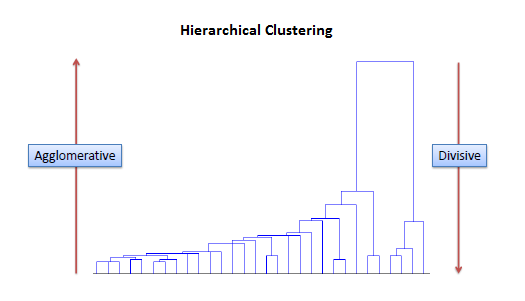
Hierarchical clustering, also known as hierarchical cluster analysis, is an algorithm that groups similar objects into groups called clusters. The endpoint is a set of clusters, where each cluster is distinct from each other cluster, and the objects within each cluster are broadly similar to each other. We can think of a hierarchical clustering is a set of nested clusters that are organized as a tree. Therefore, at the end of clustering, we can draw a dendogram which is a tree-like diagram that records the sequences of merges or splits.

Hierarchical clustering involves creating clusters that have a predetermined ordering from top to bottom. For example, all files and folders on the hard disk are organized in a hierarchy. There are two types of hierarchical clustering, Divisive and Agglomerative.

Agglomerative clustering It’s also known as AGNES (Agglomerative Nesting). It works in a bottom-up manner. That is, each object is initially considered as a single-element cluster (leaf). At each step of the algorithm, the two clusters that are the most similar are combined into a new bigger cluster (nodes). This procedure is iterated until all points are member of just one single big cluster (root). The result is a tree which can be plotted as a dendrogram.
Divisive hierarchical clustering It’s also known as DIANA (Divise Analysis) and it works in a top-down manner. The algorithm is an inverse order of AGNES. It begins with the root, in which all objects are included in a single cluster. At each step of iteration, the most heterogeneous cluster is divided into two. The process is iterated until all objects are in their own cluster. In simple words, we can say that the Divisive Hierarchical clustering is exactly the opposite of the Agglomerative Hierarchical clustering. In Divisive Hierarchical clustering, we consider all the data points as a single cluster and in each iteration, we separate the data points from the cluster which are not similar. Each data point which is separated is considered as an individual cluster. In the end, we’ll be left with n clusters.

In summary, agglomerative hierarchical clustering typically works by sequentially merging similar clusters. Divisive hierarchical clustering is done by initially grouping all the observations into one cluster, and then successively splitting these clusters.

Measures of distance (similarity)

As we learned in the K-means tutorial, we measure the (dis)similarity of observations using distance metric (i.e. Euclidean distance, Manhattan distance, etc.). However, The choice of an appropriate metric will influence the shape of the clusters, as some elements may be close to one another according to one distance and farther away according to another. For example, in a 2-dimensional space, the distance between the point $(1,0)$ and the origin $(0,0)$ is always $1$ according $1$ under maximum distance. Therefore, the choice of distance metric should be made based on theoretical concerns from the domain of study.

For text or other non-numeric data, metrics such as the Hamming distance or Levenshtein distance are often used.

Before any clustering is performed, it is required to determine the proximity matrix containing the distances between each point using a distance metric. Then, the matrix is updated to display the distance between each cluster.

After selecting a distance metric, it is necessary to determine from where distance is computed. For example, it can be computed between the two most similar parts of a cluster (single-linkage), the two least similar bits of a cluster (complete-linkage), the center of the clusters (mean or average-linkage), or some other criterion. Many linkage criteria have been developed. The linkage criterion determines the distance between sets of observations as a function of the pairwise distances between observations. As with distance metrics, the choice of linkage criteria should be made based on theoretical considerations from the domain of application. Where there are no clear theoretical justifications for the choice of linkage criteria, Ward’s method is the sensible default.

Some commonly used linkage criteria for Agglomerative clustering is described below. Do remember that in Agglomerative clustering, each data point is initially considered as a single-element cluster, meaning that when we say clusters A and B in the first step, we mean clusters with one observation in each.

Minimum (Single Link) Proximity

It computes all pairwise dissimilarities between the elements in cluster A and the elements in cluster B, and considers the smallest of these dissimilarities as a linkage criterion.

\[\min \,\{\,d(a,b):a\in A,\,b\in B\,\}\]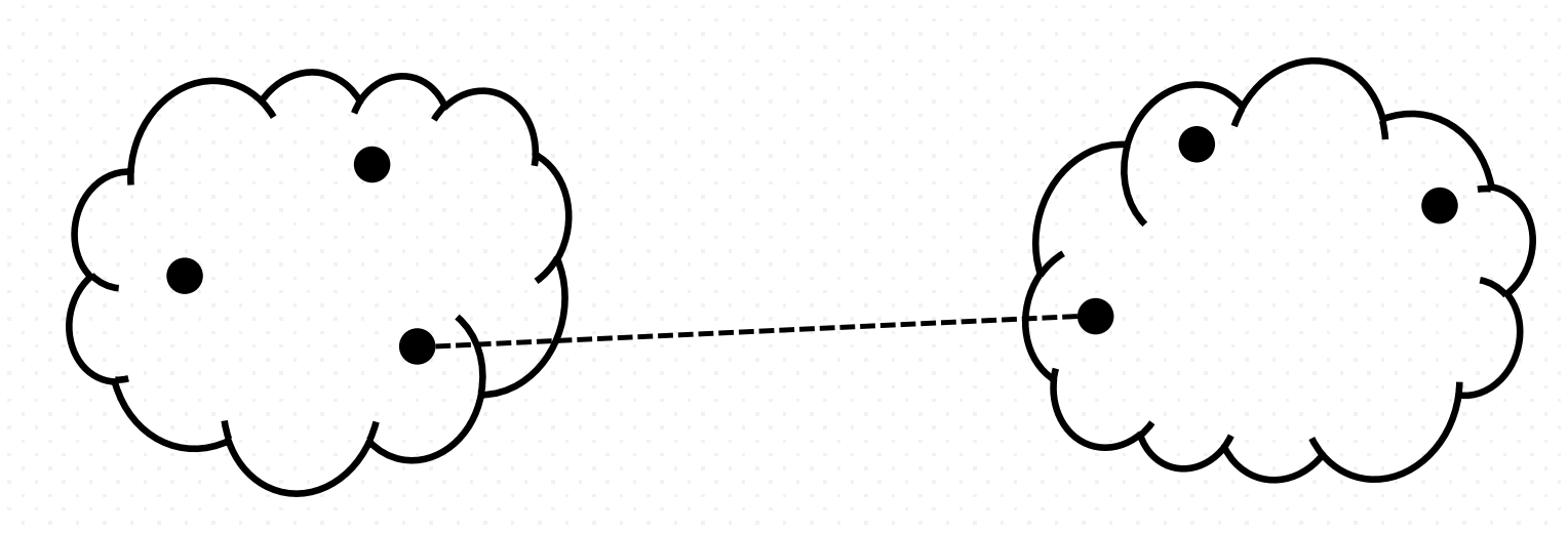

Maximum (complete-farthest distance/ complete link) Proximity

It computes all pairwise dissimilarities between the elements in cluster A and the elements in cluster B, and considers the largest value (i.e., maximum value) of these dissimilarities as the distance between the two clusters.

\[\max \,\{\,d(a,b):a\in A,\,b\in B\,\}\]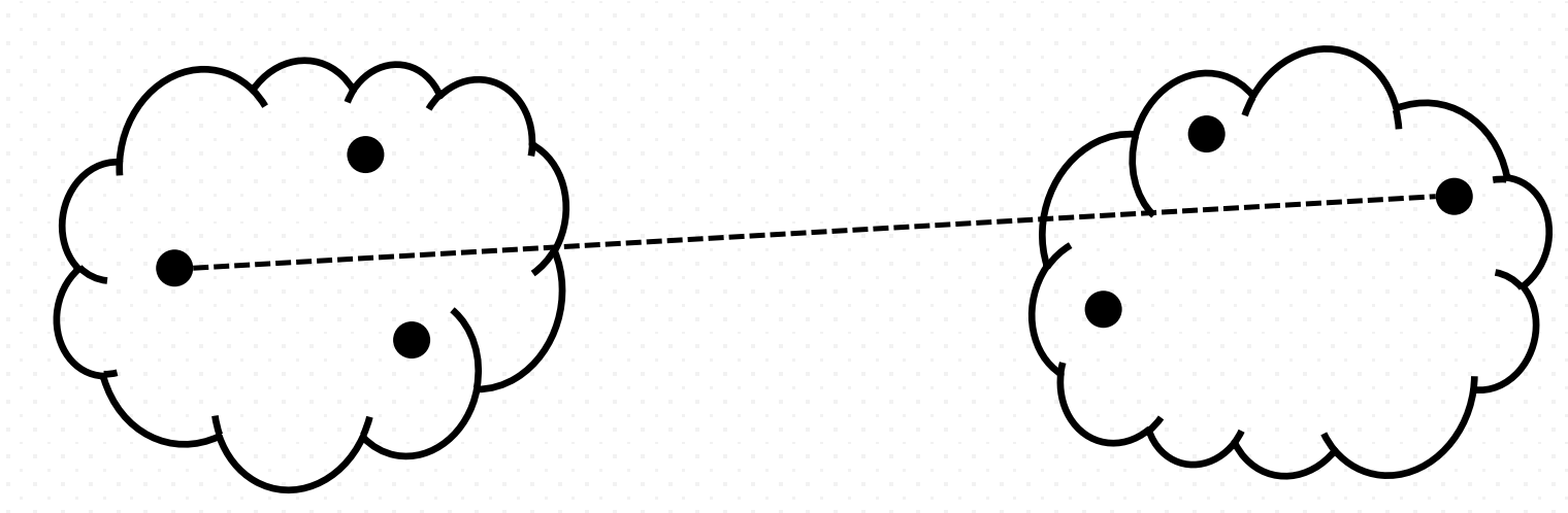

Mean or average linkage clustering

It computes all pairwise dissimilarities between the elements in cluster A and the elements in cluster B, and considers the average of these dissimilarities as the distance between the two clusters. (number of points in cluster $j$ is $n_{j}$):

\[d(A, B) = \frac{1}{n_{A}n_{B}}\sum_{a\in A} \sum_{b\in B} d(a, b)\]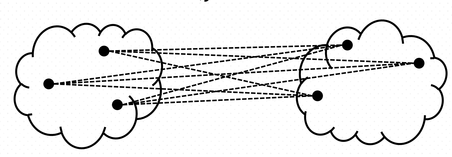

Centroid linkage clustering

It computes the dissimilarity between the centroid for cluster A and the centroid for cluster B. The distance between two clusters is the distance between the two mean vectors of the clusters. At each stage of the process we combine the two clusters that have the smallest centroid distance.

\[\|c_{A}-c_{B}\|\text{ where $c_{A}$ and $c_{B}$ are the centroids of clusters $A$ and $B$, respectively}\]

Ward’s minimum variance method

It minimizes the total within-cluster variance. At each step, the pair of clusters with minimum between-cluster distance are merged.

Ward’s method says that the distance between two clusters, A and B, is how much the sum of squares will increase when we merge them. With this method, the sum of squares starts out at zero (because every point is in its own cluster) and then grows as we merge clusters. Ward’s method keeps this growth as small as possible.

\[\Delta(A,B) = \sum_{i\in A \bigcup B} ||\overrightarrow{x_i} - \overrightarrow{m}_{A \bigcup B}||^2 - \sum_{i \in A}||\overrightarrow{x_i} - \overrightarrow{m}_A||^2 -\sum_{i \in B}||\overrightarrow{x_i}- \overrightarrow{m}_B||^2 = \frac{n_An_B}{n_A+n_B} ||\overrightarrow{m}_A- \overrightarrow{m}_B||^2\]

where $\overrightarrow{m_{j}}$ is the center of cluster $j$, and $n_{j}$ is the number of points in it. $\Delta$ is called the merging cost of combining the clusters A and B.

The distance metrics used in clustering cannot be varied with Ward, thus for non-Euclidean metrics, you need to use other linkage techniques. The Euclidean distance is the “ordinary” straight-line distance between two points in Euclidean space.

\[d(p,q) = d(q,p) = \sqrt{(q_1 -p_1)^2 + (q_2 - p_2)^2 + \cdots + (q_n -p_n)^2} = \sqrt{\sum_{i=1} (q_i-p_i)^2}\]

Like other clustering methods, when we have $n$ data points, Ward’s method starts with $n$ clusters, each containing a single object. These $n$ clusters are combined to make one cluster containing all objects. At each step, the process makes a new cluster that minimizes variance.

In order to select a new cluster at each step, every possible combination of clusters must be considered. This entire cumbersome procedure makes it practically impossible to perform by hand, making a computer a necessity for most data sets containing more than a handful of data points.

When spherical multivariate normal distributions are used, Ward’s method is excellent, which is only natural because this method is based on a sum of squares criterion. However, it must be noted that Ward’s method only performs well if an equal number of objects is drawn from each population and it looks for spherical clusters. In other words, it has difficulties with clusters of unequal diameters. Moreover, Ward’s method often leads to misclassifications when the clusters are distinctly ellipsoidal rather than spherical, that is, when the variables are correlated within a cluster.

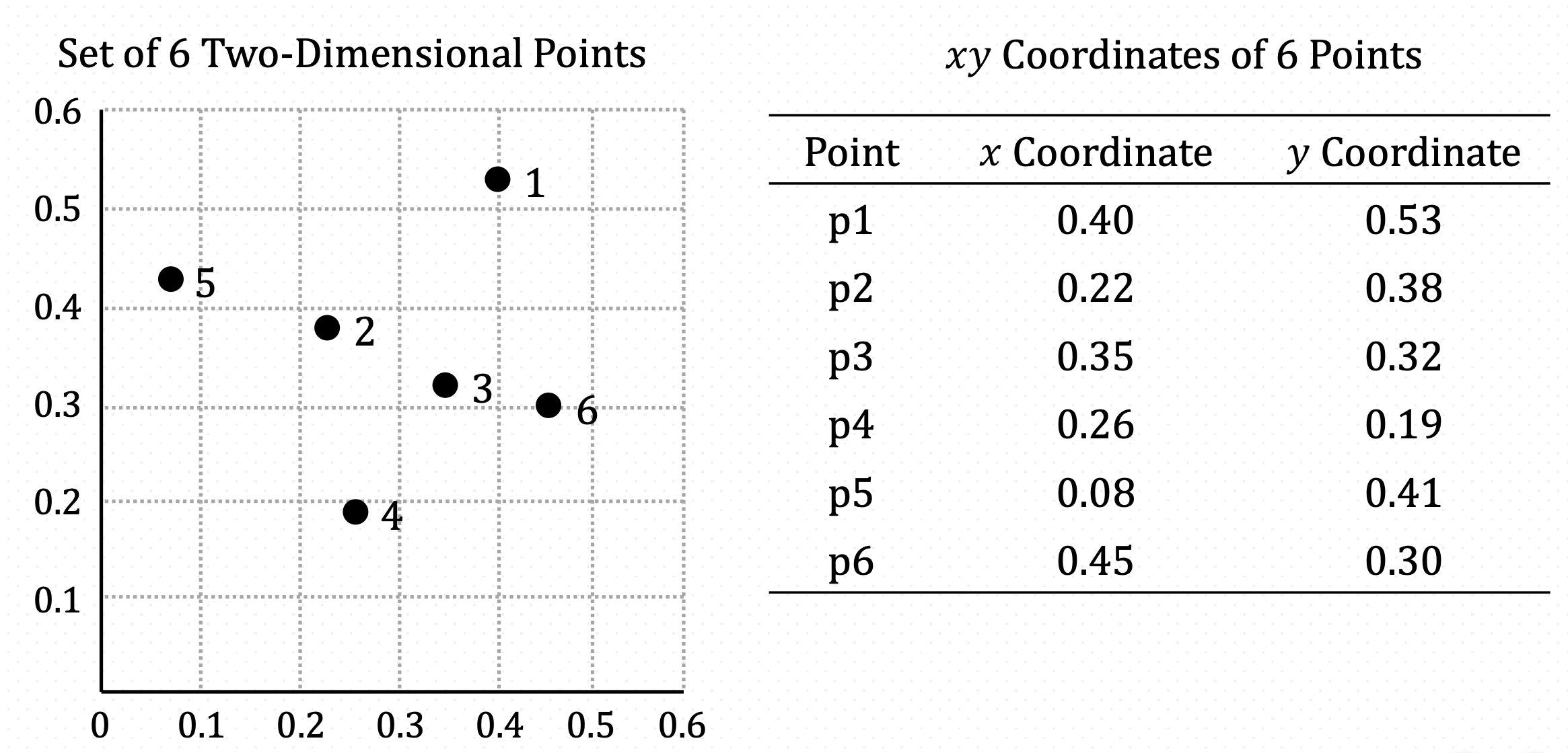
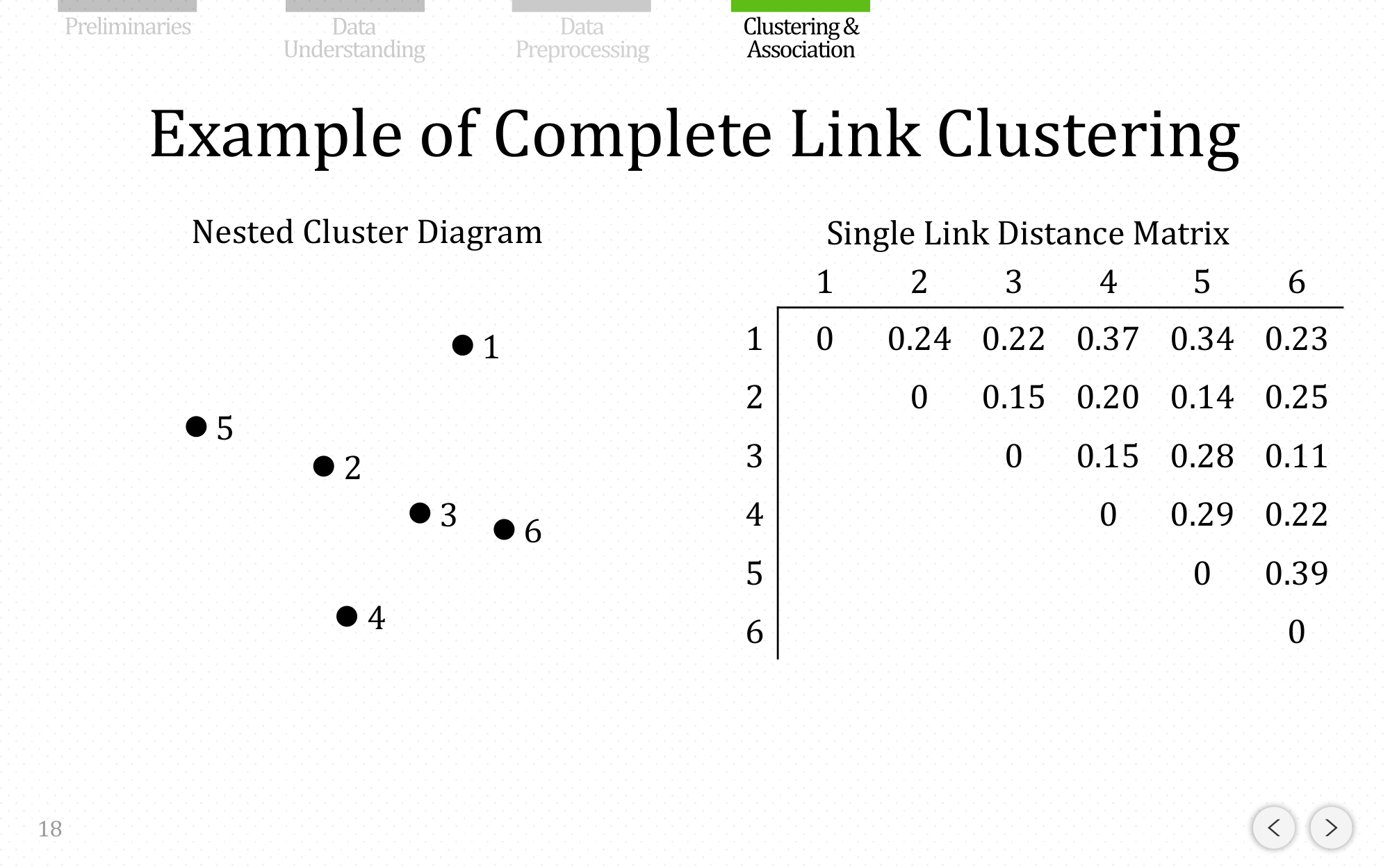
Example Data for Clustering

Let’s have one example using three different linkage method. Here, we have 6 data points with 2 variables.

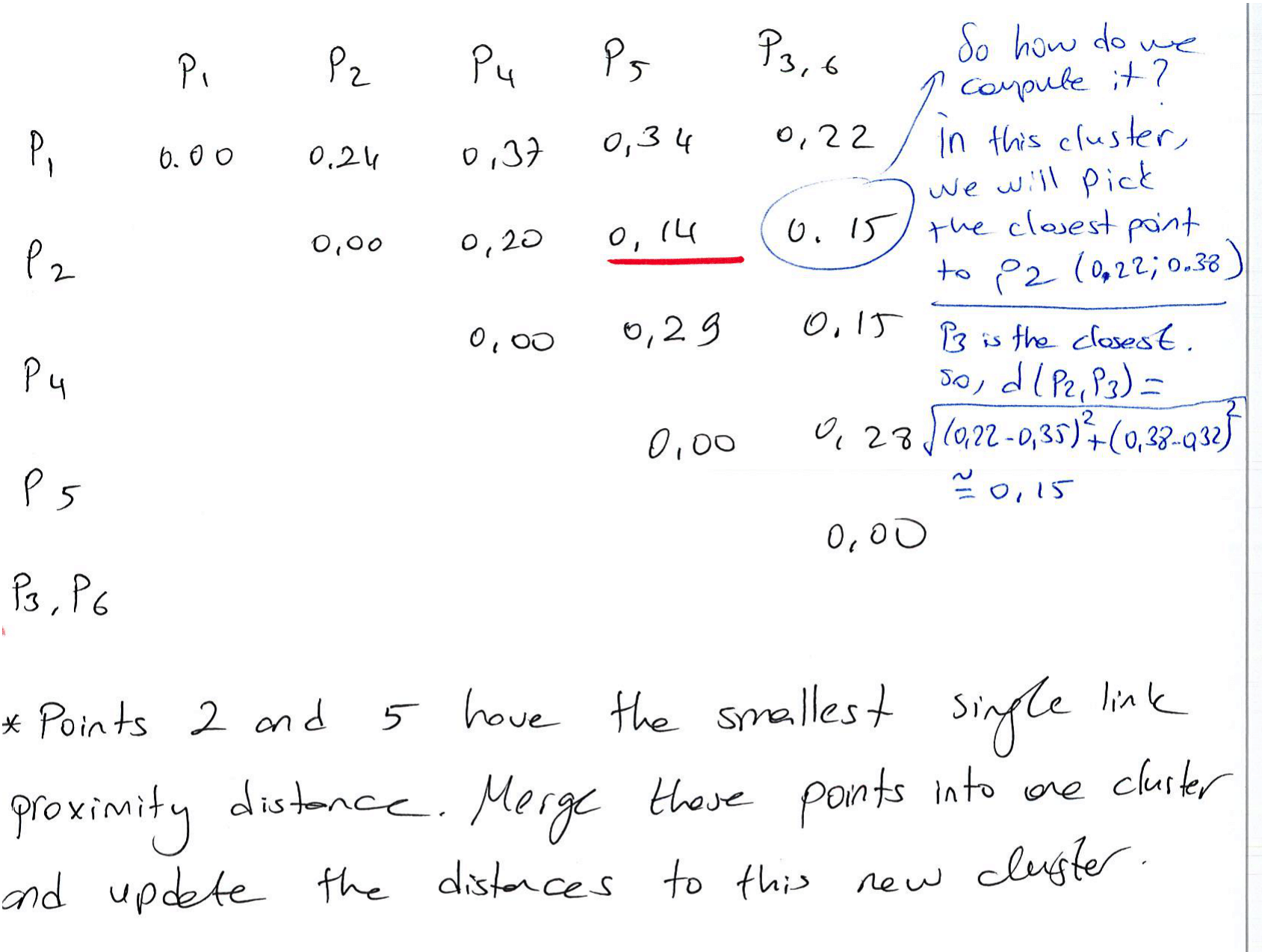
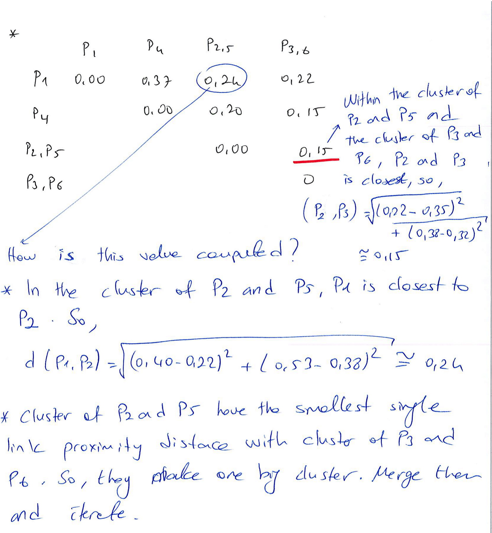
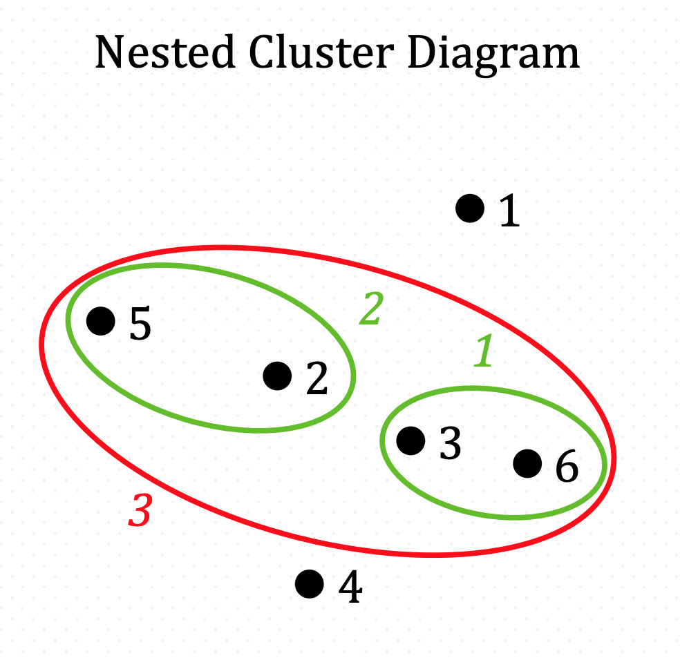
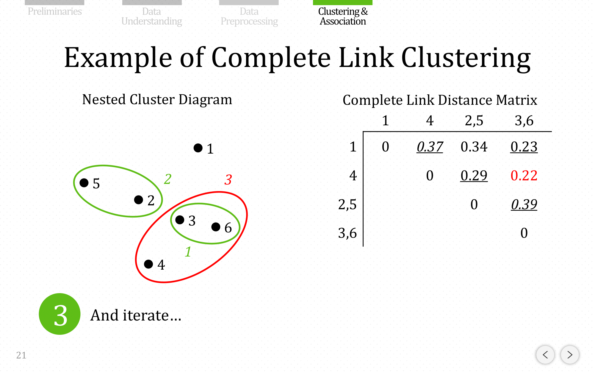
And iterate…

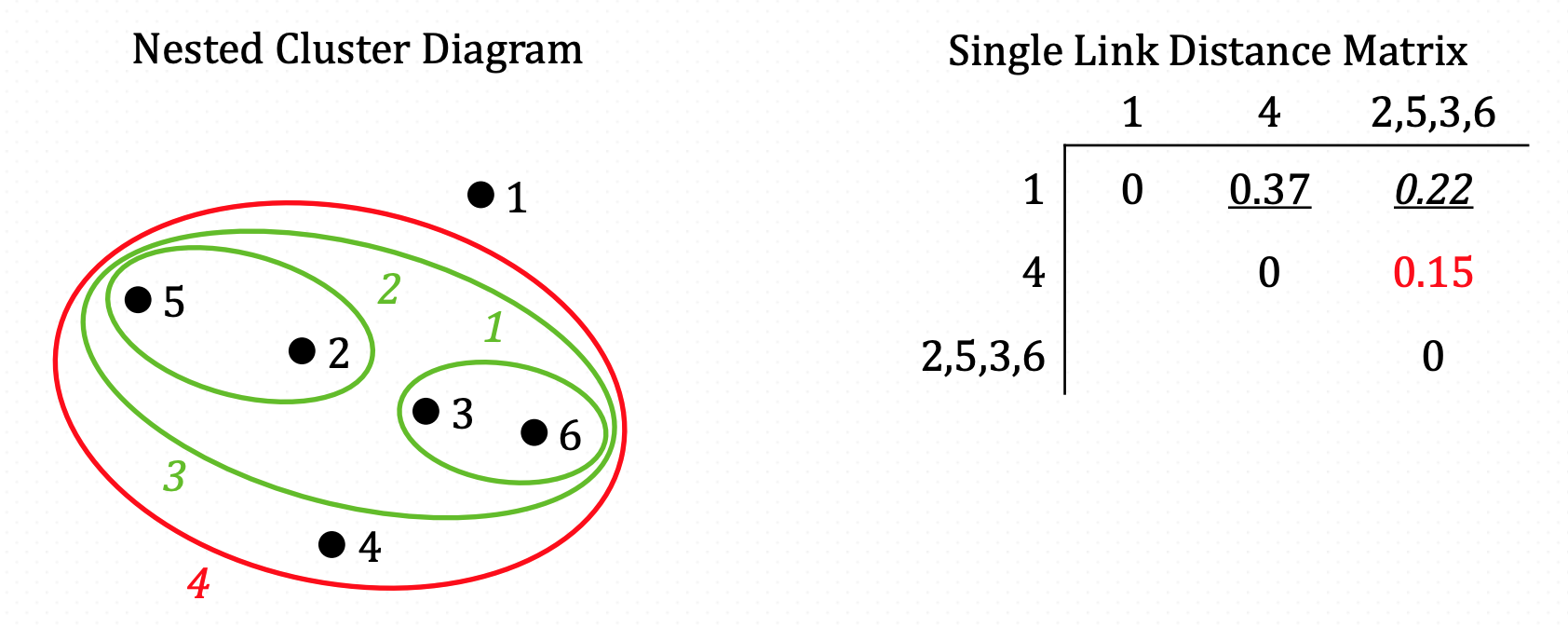
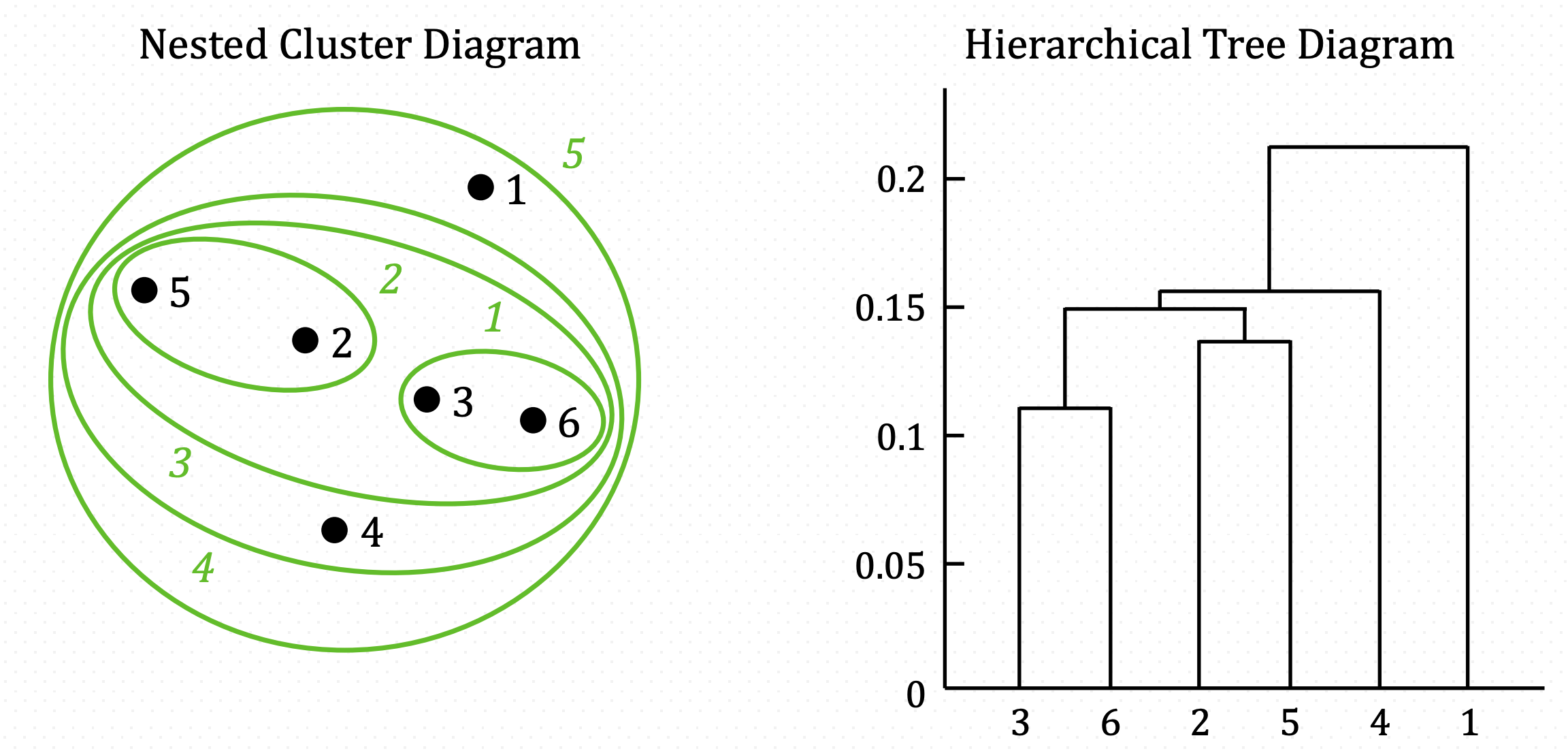
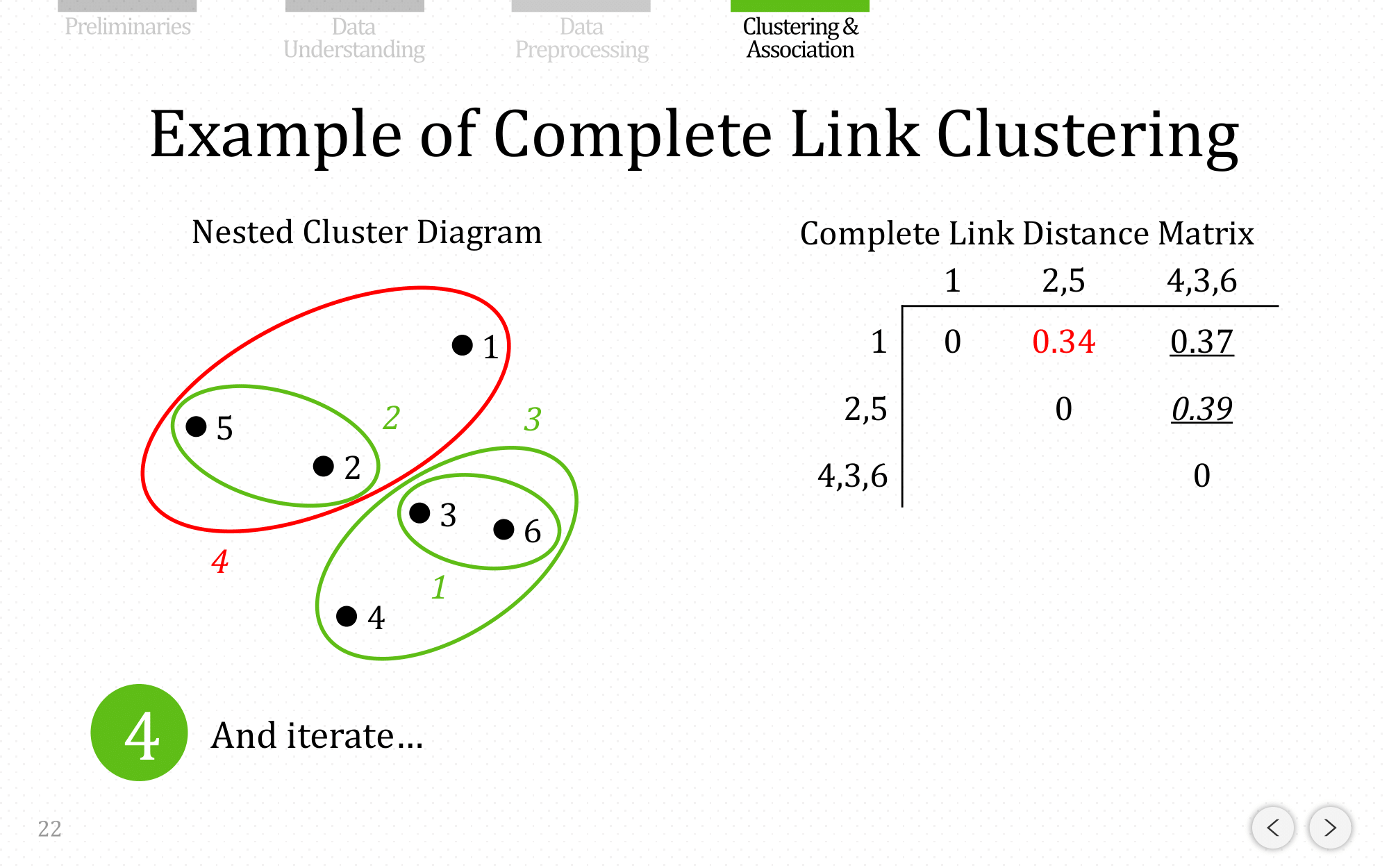
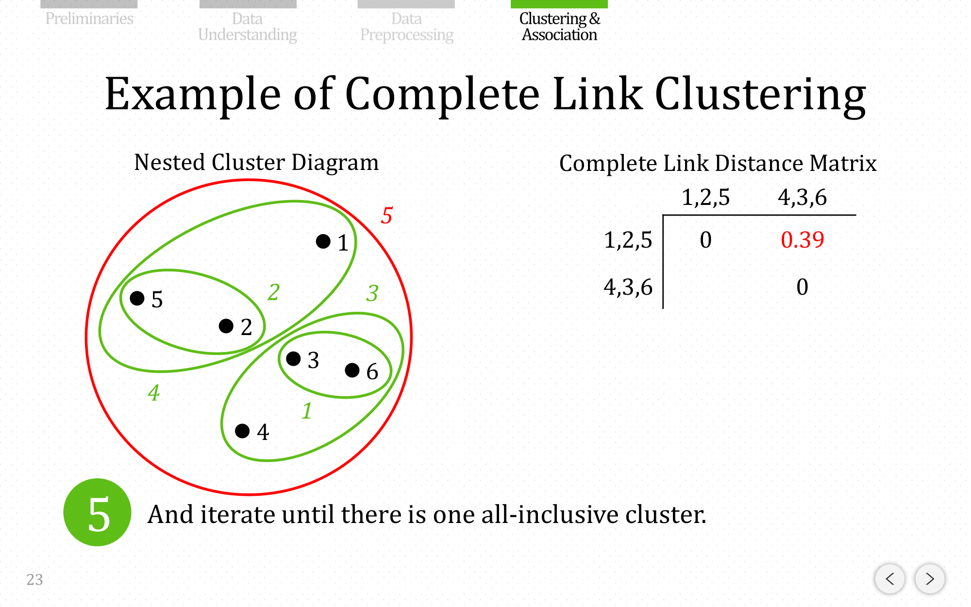
And iterate until there is one all-inclusive cluster

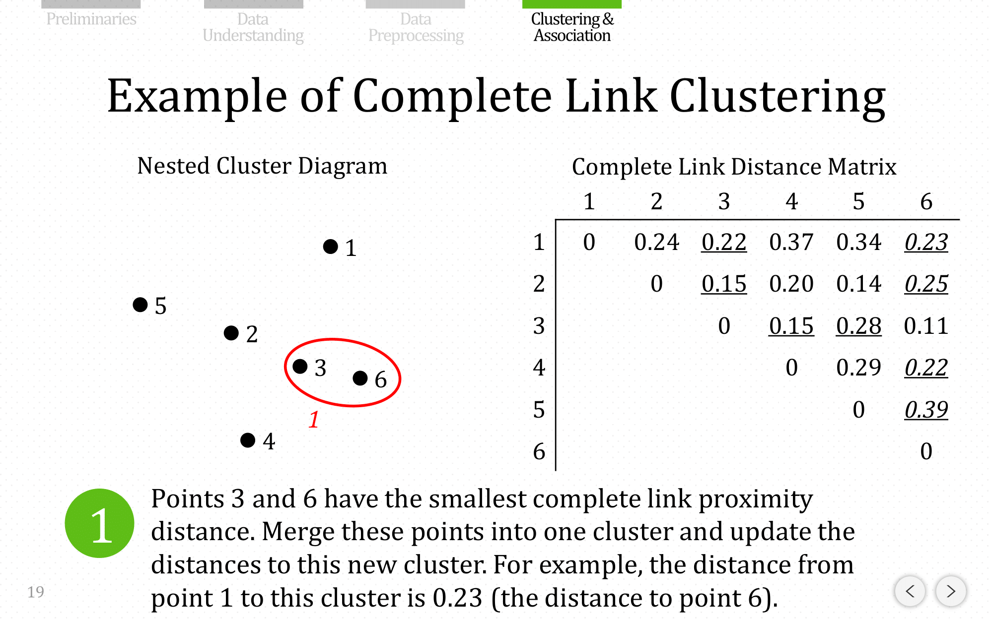
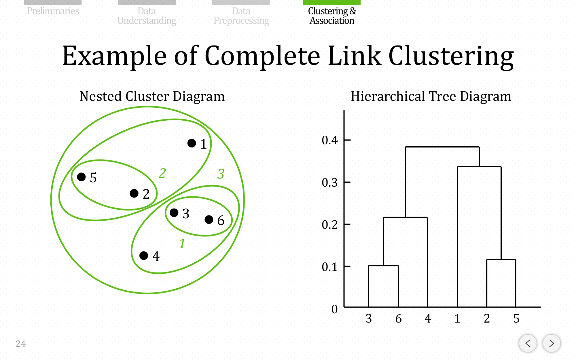
Let’s do the same example using complete linkage:

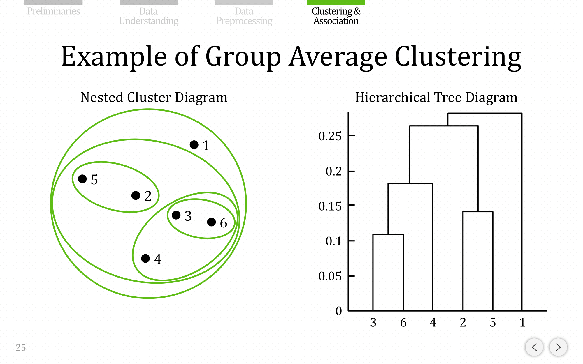
and let’s show the end result for average linkage:

Discussion of Proximity Methods

Single link is “chain-like” and good at handling nonelliptical shapes, but is sensitive to outliers.
Complete link is less susceptible to noise and outliers, but can break large clusters and favors globular shapes.
Group average is an intermediate approach between the single and complete link approaches.

Agglomerative Clustering In Scikit-Learn

import matplotlib.pyplot as plt
%matplotlib inline
import numpy as np
from sklearn.datasets import make_blobs
import pandas as pd
import scipy.cluster.hierarchy as sch
from sklearn.cluster import AgglomerativeClustering

#Let's create some data
X, y_true = make_blobs(n_samples=200, n_features=2, centers=4, cluster_std=1.6, random_state=42)
#Generate isotropic Gaussian blobs for clustering
plt.scatter(X[:, 0], X[:, 1], s=10)

#Plot the dendogram
dendrogram = sch.dendrogram(sch.linkage(X, method='ward'))

In scikit-learn, AgglomerativeClustering uses the linkage parameter to determine the merging strategy to minimize the 1) variance of merged clusters (ward), 2) average of distance between observations from pairs of clusters (average), (3) minimum distance between observations from pairs of cluster (single) or 4) maximum distance between observations from pairs of clusters (complete).

Two other parameters are useful to know. First, the affinity parameter determines the distance metric used for linkage (“euclidean”, “l1”, “l2”, “manhattan”, “cosine”, or “precomputed”. Note that when you use ward linkage, the distance metric should be euclidean). Second, n_clusters sets the number of clusters the clustering algorithm will attempt to find. That is, clusters are successively merged until there are only n_clusters remaining.

model = AgglomerativeClustering(n_clusters=4, affinity='euclidean', linkage='ward')
model.fit(X)
# AgglomerativeClustering(affinity='euclidean', compute_full_tree='auto',
#                         connectivity=None, distance_threshold=None,
#                         linkage='ward', memory=None, n_clusters=4)
y_pred = model.fit_predict(X)

plt.scatter(X[y_pred==0, 0], X[y_pred==0, 1], s=50, marker='o', color='red')
plt.scatter(X[y_pred==1, 0], X[y_pred==1, 1], s=50, marker='o', color='blue')
plt.scatter(X[y_pred==2, 0], X[y_pred==2, 1], s=50, marker='o', color='green')
plt.scatter(X[y_pred==3, 0], X[y_pred==3, 1], s=50, marker='o', color='green')

plt.show()

# Create a DataFrame with labels and varieties as columns: df
df = pd.DataFrame({'Labels': y_true, 'Clusters': y_pred})
# Create crosstab: ct
ct = pd.crosstab(df['Labels'], df['Clusters'])

# Display ct
print(ct)

Advantages and Disadvantages of Hierarchical Clustering

We choose whether to use K-means algorithm or Hierarchical Clustering depending on our problem statement and requirement. However, there are still some pros and cons to compare for both methods.

In Hierarchical Clustering, we do not need to specify the number of clusters required for the algorithm, unlike K-means (if we do not have domain knowledge) because we can stop at whatever number of clusters we find appropriate in hierarchical clustering by interpreting the dendrogram.
Hierarchical clustering is easy to implement.
Hierarchical clustering can’t handle big data well but K Means clustering can. This is because the time complexity of K Means is linear i.e. $O(n)$ while that of hierarchical clustering is quadratic i.e. $O(n^{2})$ with $n$ being the number of data points. This makes hierarchical clustering can be painfully slow and computationally expensive because it has to make several merge/split decisions.
K-Means produce tighter clusters than hierarchical clustering, especially if the clusters are hyper-spherical (like circle in 2D, sphere in 3D).
In Hierarchical Clustering, we can stop at whatever number of clusters you find appropriate in hierarchical clustering by interpreting the dendrogram. But, if we have a large dataset, it can become difficult to determine the correct number of clusters by the dendrogram because you might get something like this:

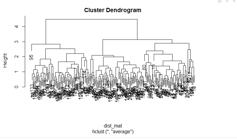
You will not be able to clearly visualize the final output. You can still use this to check at which point the item was split into different categories. K-means produces centroids which are easy to understand and use. Hierarchical clustering, on the other hand, produces a dendrogram. A dendrogram can also be very very useful in understanding your data set.
In K Means clustering, since we start with random choice of clusters, the results produced by running the algorithm multiple times might differ, while results are reproducible in Hierarchical clustering.
Hierarchical clustering is used when the variance of distribution of variables is non-spherical (one of the assumption of K means is that the distribution of variables should be spherical), it performs relatively better.
Hierarchical clustering can never undo any previous steps (no backtracking). Once the instances have been assigned to a cluster, they can no longer be moved around.
Hierarchical clustering is also sensitive to noise and outliers.
Agglomerative cluster has a “rich get richer” behavior that leads to uneven cluster sizes. In this regard, single linkage is the worst strategy, and Ward gives the most regular sizes. However, the distance metrics used in clustering cannot be varied with Ward, thus for non Euclidean metrics, average linkage is a good alternative. Single linkage, while not robust to noisy data, can be computed very efficiently and can therefore be useful to provide hierarchical clustering of larger datasets. Single linkage can also perform well on non-globular data.

Two-phase solution for clustering large datasets

When working with a large number of observations, the computations for a hierarchical cluster solution may take hours to complete, making this solution less feasible. You can get around the time issue by using two-phase clustering, which is faster and provides you with a hierarchical solution even when you are working with large datasets.

To implement the two-phase clustering solution, you process the original observations using K-means with a large number of clusters. A good rule of thumb is to take the square root of the number of observations and use that figure, but you always have to keep the number of clusters in the range of 100–200 for the second phase, based on hierarchical clustering, to work well.

from sklearn.cluster import KMeans
clustering = KMeans(n_clusters=100, n_init=10, random_state=1)
clustering.fit(Cx)

At this point, the tricky part is to keep track of what case has been assigned to what cluster derived from K-means. You can use a dictionary for such a purpose.

Kx = clustering.cluster_centers_
Kx_mapping = {case:cluster for case, cluster in enumerate(clustering.labels_)}

The new dataset is Kx (clustering.cluster_centers_), which is made up of the cluster centroids that the K-means algorithm has discovered. You can think of each cluster as a well-represented summary of the original data. If you cluster the summary now, it will be almost the same as clustering the original data.

from sklearn.cluster import AgglomerativeClustering
Hclustering = AgglomerativeClustering(n_clusters=10, affinity=‘cosine’, linkage=‘complete’)
Hclustering.fit(Kx)

You now map the results to the centroids you originally used so that you can easily determine whether a hierarchical cluster is made of certain K-means centroids. The result consists of the observations making up the K-means clusters having those centroids.

H_mapping = {case:cluster for case, cluster in enumerate(Hclustering.labels_)}
final_mapping = {case:H_mapping[Kx_mapping[case]] for case in Kx_mapping}

Now you can evaluate the solution you obtained using a similar confusion matrix as you did before for both K-means and hierarchical clustering.

ms = np.column_stack((ground_truth, [final_mapping[n] for n in range(max(final_mapping)+1)]))
df = pd.DataFrame(ms, columns = [‘Ground truth’,’Clusters’])
pd.crosstab(df[‘Ground truth’], df[‘Clusters’], margins=True)

The result proves that this approach is a viable method for handling large datasets or even big data datasets, reducing them to a smaller representations and then operating with less scalable clustering, but more varied and precise techniques.

REFERENCES

← → Top