on
5 mins to read.
RGB to Grayscale Conversion
Consider a color image, given by its red, green, blue components R, G, B. The range of pixel values is often 0 to 255. Color images are represented as multi-dimensional arrays - a collection of three two-dimensional arrays, one each for red, green, and blue channels. Each one has one value per pixel and their ranges are identical. For grayscale images, the result is a two-dimensional array with the number of rows and columns equal to the number of pixel rows and columns in the image.
We present some methods for converting the color image to grayscale:
import cv2
import numpy as np
import matplotlib.pyplot as plt
%matplotlib inline

img_path = 'img_grayscale_algorithms.jpg'

img = cv2.imread(img_path)
print(img.shape)
#(1300, 1950, 3)

#Matplotlib EXPECTS RGB (Red Greed Blue)
#but...
#OPENCV reads as Blue Green Red

#we need to transform this in order that Matplotlib reads it correctly
fix_img = cv2.cvtColor(img, cv2.COLOR_BGR2RGB)
plt.imshow(fix_img)

#Let's extract the three channels
R, G, B = fix_img[:,:,0], fix_img[:,:,1],fix_img[:,:,2]

Weighted average
This is the grayscale conversion algorithm that OpenCV’s cvtColor() use (see the documentation)
The formula used is:
\[Y = 0.299\times R + 0.587 \times G + 0.114 \times B\]Y = 0.299 * R + 0.587 * G + 0.114 * B
print(Y)
# [[ 85.967 88.967 92.967 ... 27.85 27.85 27.85 ]
# [ 83.967 86.967 89.967 ... 27.85 27.85 27.85 ]
# [ 81.956 83.956 86.967 ... 26.85 26.85 26.85 ]
# ...
# [121.015 112.243 108.998 ... 108.02 108.792 108.792]
# [120.086 111.086 108.727 ... 107.02 106.792 106.792]
# [118.086 111.086 109.727 ... 105.02 104.792 105.792]]
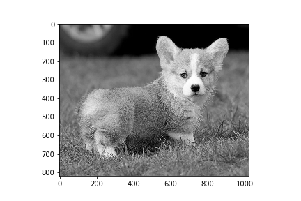
plt.imshow(Y, cmap='gray')
plt.savefig('image_weighted_average_byhand.png')

Let’s compare it with the original function in OpenCV:
img_gray = cv2.imread(img_path, cv2.IMREAD_GRAYSCALE)
print(img_gray)
# [[ 86  89  93 ...  28  28  28]
#  [ 84  87  90 ...  28  28  28]
#  [ 82  84  87 ...  27  27  27]
#  ...
#  [121 112 109 ... 108 109 109]
#  [120 111 109 ... 107 107 107]
#  [118 111 110 ... 105 105 106]]

plt.imshow(img_gray, cmap='gray')
plt.savefig('image_weighted_average_OPENCV.png')

Average method
Average method is the most simple one. You just have to take the average of three colors. Since its an RGB image, so it means that you have add R with G with B and then divide it by 3 to get your desired grayscale image.
grayscale_average_img = np.mean(fix_img, axis=2)
# (axis=0 would average across pixel rows and axis=1 would average across pixel columns.)
print(grayscale_average_img)
# [[82.         85.         89.         ... 26.         26.
#   26.        ]
#  [80.         83.         86.         ... 26.         26.
#   26.        ]
#  [77.66666667 79.66666667 83.         ... 25.         25.
#   25.        ]
#  ...
#  [92.         83.66666667 81.33333333 ... 81.         81.33333333
#   81.33333333]
#  [90.66666667 81.66666667 80.         ... 80.         79.33333333
#   79.33333333]
#  [88.66666667 81.66666667 81.         ... 78.         77.33333333
#   78.33333333]]

plt.imshow(grayscale_average_img, cmap='gray')
plt.savefig('image_average_method.png')

Since the three different colors have three different wavelength and have their own contribution in the formation of image, so we have to take average according to their contribution, not done it averagely using average method. Right now what we are doing is 33% of Red, 33% of Green, 33% of Blue. We are taking 33% of each, that means, each of the portion has same contribution in the image. But in reality that is not the case. The solution to this has been given by luminosity method.
The luminosity method
This method is a more sophisticated version of the average method. It also averages the values, but it forms a weighted average to account for human perception. Through many repetitions of carefully designed experiments, psychologists have figured out how different we perceive the luminance or red, green, and blue to be. They have provided us a different set of weights for our channel averaging to get total luminance. The formula for luminosity is:
\[Z = 0.2126\times R + 0.7152 G + 0.0722 B\]According to this equation, Red has contribute 21%, Green has contributed 72% which is greater in all three colors and Blue has contributed 7%.
Z = 0.2126 * R + 0.7152 * G + 0.0722 * B
print(Z)
# [[ 84.7266  87.7266  91.7266 ...  27.404   27.404   27.404 ]
#  [ 82.7266  85.7266  88.7266 ...  27.404   27.404   27.404 ]
#  [ 81.0166  83.0166  85.7266 ...  26.404   26.404   26.404 ]
#  ...
#  [128.2216 119.366  115.8674 ... 114.2874 115.143  115.143 ]
#  [127.2898 118.2898 115.719  ... 113.2874 113.143  113.143 ]
#  [125.2898 118.2898 116.719  ... 111.2874 111.143  112.143 ]]

plt.imshow(Z, cmap='gray')
plt.savefig('image_luminosity_method.png')
As you can see here, that the image has now been properly converted to grayscale using the luminosity method. As compare to the result of average method, this image is more brighter than average method.