Batch Normalization

Normalizing the input of your network is a well-established technique for improving the convergence properties of a network. A few years ago, a technique known as batch normalization was proposed to extend this improved loss function topology to more of the parameters of the network.

The method consists of adding an operation in the model just before the activation function of each layer, simply, zero-centering and normalizing the inputs of that particular layer and then scaling and shifting the result using two new parameters per layer (one for scaling, the other for shifting). In other words, this operation lets the model learn the optimal scale and mean of the inputs for each layer.

In order to zero-center and normalize the inputs, the algorithm needs to estimate the inputs’ mean and standard deviation. It does so by evaluating the mean and standard deviation of the inputs over the current mini-batch (hence the name “Batch Normalization”).

It is a widely used technique for normalizing the internal representation of data on models that can lead to substantial reduction in convergence time. It also helps to reduce something called “internal covariate shift” of the network.

It introduces some noise into the network, so it can regularize the model a bit. However, regularization is a side effect of Batch Normalization, rather than the main objective.

However, there is a one drawback of Batch Normalization, which is that it makes the training slower due to extra computations required at each layer.

Batch Normalization Equations

For a given input batch $\phi$ of size $(N,F)$ going through a hidden layer of size $D$, some weights $w$ of size $(F,D)$ and a bias $b$ of size $(D)$, we first do an affine transformation $X = Z \cdot W + b$ where $X$ contains the results of the linear transformation (size $(N,D)$).

Then, a Batch Normalization layer is given a batch of $N$ examples, each of which is a $D$-dimensional vector in a mini-batch $\phi$, where $D$ is the number of hidden units. We can represent the inputs as a matrix $X \in R^{N \times D}$ where each row $x_{i}$ is a single example. Each example $x_{i}$ is normalized by

Every component of $\hat{x}$ has zero mean and unit variance. However, we want hidden units to have different distributions. In fact, this would perform poorly for some activation functions such as the sigmoid function. Thus, we’ll allow our normalization scheme to learn the optimal distribution by scaling our normalized values by $\gamma$ and shifting by $\beta$:

In other words, we’ve now allowed the network to normalize a layer into whichever distribution is most optimal for learning.

• $\mu_\phi \in R^{1 \times D}$: is the empirical mean of each input dimension across the whole mini-batch.
• $\sigma_\phi \in R^{1 \times D}$ is the empirical standard deviation of each input dimension across the whole mini-batch.
• $N$ is the number of instances in the mini-batch
• $\hat{x_i}$ is the zero-centered and normalized input.
• $\gamma \in R^{1 \times D}$ is the scaling parameter for the layer.
• $\beta \in R^{1 \times D}$ is the shifting parameter (offset) for the layer.
• $\epsilon$ is added for numerical stability, just in case ${\sigma_\phi}^2$ turns out to be 0 for some estimates. This is also called a smoothing term.
• $y_i$ is the output of the BN operation. It is the scaled and shifted version of the inputs. $y_{i}=BN_{\gamma,\beta}(x_{i})$

NOTE: the authors did something really clever. They realized that by normalizing the output of a layer they could limit its representational power and, therefore, they wanted to make sure that the Batch Norm layer could fall back to the identity function. If $\beta$ is set to $\mu_\phi$ and $\gamma$ to $\sqrt{\sigma_{\phi}^{2} + \epsilon}$, $\hat{x_i}$ equals to $x_i$, thus working as an identity function. That means that the network has the ability to ignore the Batch Norm layer if that is the optimal thing to do and introducing batch normalization alone would not reduce the accuracy because the optimizer still has the option to select no normalization effect using the identity function and it would be used by the optimizer to only improve the results.

NOTE: $\gamma$ and $\beta$ are learnable parameters that are initialized with $\gamma =1$ and $\beta = 0$.

NOTE: Batch Normalization is done individually at every hidden unit.

CORRECTION

Note that, all the expressions above implicitly assume broadcasting as $X$ is of size $(N,D)$ and both $\mu_{\phi}$ and $\sigma_{\phi}^{2}$ have size equal to $(D)$. A more correct expression would be

where

and

with $i = 1\dots ,N$ and $l = 1,\dots ,D$.

However, for the rest, we will stick to original paper’s definitions.

Inference

During testing time, the implementation of batch normalization is quite different.

While it is acceptable to compute the mean and variance on a mini-batch when we are training the network, the same does not hold on test time. When the batch is large enough, its mean and variance will be close to the population’s. The non-deterministic mean and variance has regularizing effects. On test time, we want the model to be deterministic.

At test time, there is no mini-batch to compute the empirical mean and standard deviation, so instead you simply use the whole training set’s mean and standard deviation, meaning that population instead of the mini-batch statistics.

We calculate “population average” of mean and variances after training, using all the batches’ means and variances, and at inference time, we fix the mean and variance to be this value and use it in normalization. This provides more accurate value of mean and variance.

Then, at inference time, using those population mean and variance, we do normalization:

But, sometimes, it is difficult to keep track of all the mini-batch mean and variances. In such cases, exponentially weighted “moving average” can be used as global statistics to update population mean and variance:

Here $\alpha$ is the “momentum” given to previous moving statistic, around $0.99$, and those with $\phi$ subscript are mini-batch mean and mini-batch variance. This is the implementation found in most libraries, where the momentum can be set manually.

Backward Pass

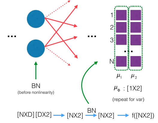
We follow the dark arrows for the forward pass and then we backpropagate the error using the red ones. The dimension of the output of each node is displayed on top of each node.

Let $L$ be the loss function and we are given $\frac{\partial L}{\partial Y} \in R^{N \times D}$, the gradient of loss with respect to $Y$. Our goal is to compute three gradients:

1. $\frac{\partial L}{\partial \gamma} \in R^{1 \times D}$ to perform gradient descent update on $\gamma$.
2. $\frac{\partial L}{\partial \beta} \in R^{1 \times D}$ to perform gradient descent update on $\beta$.
3. $\frac{\partial L}{\partial X} \in R^{N \times D}$ to pass on the gradient signal to lower layers.

Both $\frac{\partial L}{\partial \gamma}$ and $\frac{\partial L}{\partial \beta}$ are straightforward to compute. Let $y_{i}$ be the $i$-th row of $Y$.

Notice that we sum from 1 to N, because we are working with batches.

Similarly, we compute the gradient with respect to $\beta$ as follows:

What we need to compute next is the partial derivative of the loss with respect to the input $x_{i}$. So, the previous layers can compute their gradients and update their parameters. We need to gather all the expressions where $x_{i}$ is used that has influence on $y_{i}$.

$x_{i}$ is used to compute $\hat{x_{i}}$, $\mu_{\phi}$ and $\sigma_{\phi}^{2}$, therefore,

Let’s compute and simplify each of these terms individually

The first one is the easiest to derive:

and

Therefore,

The very next expression is a bit longer.

We know that

\(\hat{x_i} = \frac{x_i-{\mu_\phi}}{\sqrt{\sigma_{\phi}^{2} + \epsilon}}\).

Here $(x_i-{\mu_{\phi}})$ is constant, so:

As what happened with the gradients of $\gamma$ and $\beta$, to compute the gradient of $\sigma_{\phi}^{2}$, we need to sum over the contributions of all elements from the batch. The same happens to the gradient of $\mu_{\phi}$ as it is also a $D$-dimensional vector. However, this time, $\sigma_{\phi}^{2}$ is also a function of $\mu_{\phi}$.

Let’s compute the missing partials one at a time.

From

we compute

and from

we calculate

We already know $\frac{\partial L}{\partial \hat{x_{i}}}$ and $\frac{\partial L}{\partial \sigma_{\phi}^{2}}$. So, let’s put them all together:

It seems complicated but it is actually super easy to simplify. Since $\sum_{i=1}^{N} (x_{i} - \mu_\phi) = 0$, the second term of this expression will be 0. Then,

Now, we can easily compute:

We still have some missing gradients which are really easy to calculate:

since

and

since

So,

When we substitute the partial derivatives into and do some simplifications using the fact that

then, we will have:

This is a simpler expression. Translating this to python, we can end up with a much more compact method.

Python Implementation

Forward Pass:

 
def batchnorm_forward(X, gamma, beta, eps):
  # mini-batch mean
  mu_phi = np.mean(x, axis=0)

  # mini-batch variance
  std_phi = np.sqrt(np.mean((X - mean) ** 2, axis=0))
  inv_std_phi = 1.0 / std 

  # normalize
  X_hat = (X - mu_phi) * inv_std_phi

  # scale and shift
  out = gamma * X_hat + beta

  # Store some variables that will be needed for the backward pass
  cache = (gamma, X_hat, inv_std_phi)

  return out, cache

Backward Pass:

 
def batchnorm_backward(dout, cache):
  N, D = dout.shape
  gamma, X_hat, inv_std_phi = cache

  dbeta = np.sum(dout, axis=0)
  dgamma = np.sum(X_hat * dout, axis=0)
  dX = (gamma*inv_std_phi/N) * (N*dout - X_hat*dgamma - dbeta)

  return dX, dgamma, dbeta

Batch Normalization in Tensorflow

When training, the moving mean and moving variance need to be updated. By default the update ops are placed in tf.GraphKeys.UPDATE_OPS, so they need to be executed alongside the train_op. Also, be sure to add any batch normalization ops before getting the update_ops collection. Otherwise, update_ops will be empty, and training/inference will not work properly. For example:

 
import tensorflow as tf
# ...
# declare a placeholder to tell the network if it is in training time or inference time 
is_train = tf.placeholder(tf.bool, name="is_train");
# ...
x_norm = tf.layers.batch_normalization(x, 
                                       center=True,
                                       scale=True,
                                       training=is_train)
# ...
update_ops = tf.get_collection(tf.GraphKeys.UPDATE_OPS)
with tf.control_dependencies(update_ops):
    train_op = optimizer.minimize(loss)

NOTE: In Tensorflow, moving mean is initialized from zero and moving variance is initialized from one.

Where to Insert Batch Norm Layers?

Batch normalization may be used on the inputs to the layer before or after the activation function in the previous layer. It may be more appropriate after the activation function if for s-shaped functions like the hyperbolic tangent and logistic function. It may be appropriate before the activation function for activations that may result in non-Gaussian distributions like the rectified linear activation function, the modern default for most network types, as the authors of the original paper puts: ‘The goal of Batch Normalization is to achieve a stable distribution of activation values throughout training, and in our experiments we apply it before the nonlinearity since that is where matching the first and second moments is more likely to result in a stable distribution’.

Advantages of Batch Normalization

• reduces internal covariate shift
• improves the gradient flow
• more tolerant to saturating nonlinearities because it is all about the range of values fed into those activation functions.
• reduces the dependence of gradients on the scale of the parameters or their initialization (less sensitive to weight initialization)
• allows higher learning rates because of less danger of exploding/vanishing gradients.
• acts as a form of regularization
• all in all accelerates neural network convergence.

Don’t Use With Dropout

Batch normalization offers some regularization effect, reducing generalization error, perhaps no longer requiring the use of dropout for regularization. Further, it may not be a good idea to use batch normalization and dropout in the same network. The reason is that the statistics used to normalize the activations of the prior layer may become noisy given the random dropping out of nodes during the dropout procedure.

REFERENCES

1. https://medium.com/deeper-learning/glossary-of-deep-learning-batch-normalisation-8266dcd2fa82
2. https://kratzert.github.io/2016/02/12/understanding-the-gradient-flow-through-the-batch-normalization-layer.html
3. https://wiseodd.github.io/techblog/2016/07/04/batchnorm/
4. http://cthorey.github.io./backpropagation/
5. https://r2rt.com/implementing-batch-normalization-in-tensorflow.html