Bag-of-Words and TF-IDF Tutorial

In information retrieval and text mining, TF-IDF, short for term-frequency inverse-document frequency is a numerical statistics (a weight) that is intended to reflect how important a word is to a document in a collection or corpus. It is based on frequency.

The TF-IDF is a product of two statistics term: tern frequency and inverse document frequency. There are various ways for determining the exact values of both statistics.

Before jumping to TF-IDF, let’s first understand Bag-of-Words (BoW) model

Bag-of-Words (BoW) model

BoW model creates a vocabulary extracting the unique words from document and keeps the vector with the term frequency of the particular word in the corresponding document. Simply term frequency refers to number of occurences of a particular word in a document. BoW is different from Word2vec. The main difference is that Word2vec produces one vector per word, whereas BoW produces one number (a wordcount).

For example:

1. John likes to watch movies. Mary likes movies too.
2. Mary also likes to watch football games.

Based on these two documents, we can construct a list for each document:

1. ["John", "likes", "to", "watch"" movies", "Mary", "likes", "movies", "too"]
2. ["Mary", "also", "likes", "to", "watch", "football", "games"]

Representing each bag-of-words as a JSON object, we get:

BOW1 = { "John": 1, "likes": 2, "to": 1, "watch": 1, "movies": 2, "Mary": 1, "too": 1}

and

BOW2 = {"Mary": 1, "also": 1, "likes": 1, "to": 1, "watch": 1, "football": 1, "games": 1}

where each key is the word and each value is the number of occurences of that word in the given text documents.

The drawbacks of Bag-of-Words model are:

1. The term ordering is not considered
2. The rareness of term is not considered
3. It results in extremely large feature dimensions and sparse vectors.

BoW model in Sci-kit Learn

We will use CountVectorizer of Sci-kit Learn to convert a collection of text documents to a matrix of token counts:

 
import pandas as pd
from sklearn.feature_extraction.text import CountVectorizer

corpus = ['John likes to match movies. Mary likes movies too.', 
          'Mary also likes to watch a football game.']

vectorizer = CountVectorizer(analyzer = "word", 
                             lowercase=True, 
                             tokenizer = None, 
                             preprocessor = None, 
                             stop_words = None, 
                             max_features = 5000)

# CountVectorizer(analyzer='word', binary=False, decode_error='strict',
#                 dtype=<class 'numpy.int64'>, encoding='utf-8', input='content',
#                 lowercase=True, max_df=1.0, max_features=5000, min_df=1,
#                 ngram_range=(1, 1), preprocessor=None, stop_words=None,
#                 strip_accents=None, token_pattern='(?u)\\b\\w\\w+\\b',
#                 tokenizer=None, vocabulary=None)

# (set lowercase=false if you don’t want lowercasing)
#performs tokenization (converts raw text to smaller units of text)
#uses word level tokenization (meaning each word is treated as a separate token)
#ignores single characters during tokenization such as 'a' and 'I'

The default tokenization in CountVectorizer removes all special characters, punctuation and single characters. If this is not the behavior you desire, and you want to keep punctuation and special characters, you can provide a custom tokenizer to CountVectorizer.

You can also use a custom stop word list that you provide, which we will see an example below!

 
# convert the documents into a document-term matrix
wm = vectorizer.fit_transform(corpus)
print(wm.todense())

# [[0 0 0 1 2 1 1 2 1 1 0]
#  [1 1 1 0 1 1 0 0 1 0 1]]

Notice that here we have 11 unique words. So we have 11 columns. Each column in the matrix represents a unique word in the vocabulary, while each row represents the document in our dataset.

 
#shape of count vector: 2 docs and 11 unique words (columns)!
wm.shape
# (2, 11)

# show resulting vocabulary; the numbers are not counts, they are the position in the sparse vector
vocabulary = vectorizer.vocabulary_
print(vocabulary)

# {'john': 3, 'likes': 4, 'to': 8, 'match': 6, 'movies': 7, 'mary': 5, 'too': 9, 'also': 0, 'watch': 10, 'football': 1, 'game': 2}

tokens = vectorizer.get_feature_names()
print(tokens)

# ['also', 'football', 'game', 'john', 'likes', 'mary', 'match', 'movies', 'to', 'too', 'watch']

# create an index for each row
doc_names = ['Doc{:d}'.format(idx) for idx, _ in enumerate(wm)]
df = pd.DataFrame(data=wm.toarray(), index=doc_names,
                  columns=tokens)
df

How to provide stop words in a list?

 
vectorizer = CountVectorizer(analyzer = "word", 
                             lowercase=True, 
                             tokenizer = None, 
                             preprocessor = None, 
                             stop_words = ['to', 'too'],
                             max_features = 5000)

# convert the documents into a document-term matrix
wm = vectorizer.fit_transform(corpus)
print(wm.shape)
#(2, 9)

vocabulary = vectorizer.vocabulary_
print(vocabulary)
#{'john': 3, 'likes': 4, 'match': 6, 'movies': 7, 'mary': 5, 'also': 0, 'watch': 8, 'football': 1, 'games': 2}

tokens = vectorizer.get_feature_names()
print(tokens)
#['also', 'football', 'games', 'john', 'likes', 'mary', 'match', 'movies', 'watch']


#To check the stop words that are being used (when explicitly specified), simply access 
stopWords = vectorizer.stop_words
print(stopWords)
#['to', 'too']

In this example, we provide a list of words that act as our stop words. Notice that the shape has gone from (2,11) to (2,9) because of the stop words that were removed, ['to', 'too']. Note that we can actually load stop words directly from a file into a list and supply that as the stop word list. One of the lists is given in https://github.com/kavgan/nlp-in-practice/blob/master/tf-idf/resources/stopwords.txt

we can also use min_df and max_df arguments to get rid of some words.

we can ignore words that are too common with max_df. max_df looks at how many documents contained a term, and if it exceeds the max_df threshold, then it is eliminated from consideration. The MAX_DF value can be an absolute value (e.g. 1, 2, 3, 4) or a value representing proportion of documents (e.g. 0.85 meaning, ignore words appeared in 85% of the documents as they are too common).

BoW model by hand

 
#https://gist.github.com/edubey/c52a3b34541456a76a2c1f81eebb5f67

import numpy
import re

'''
Tokenize each the sentences, example
Input : "John likes to watch movies. Mary likes movies too"
Ouput : "John","likes","to","watch","movies","Mary","likes","movies","too"
'''
def tokenize(sentences):
    words = []
    for sentence in sentences:
        w = word_extraction(sentence)
        words.extend(w)
        
    words = sorted(list(set(words)))
    return words

def word_extraction(sentence):
    ignore = ['a', "the", "is"]
    words = re.sub("[^\w]", " ",  sentence).split()
    cleaned_text = [w.lower() for w in words if w not in ignore]
    return cleaned_text    
    
def generate_bow(allsentences):    
    vocab = tokenize(allsentences)
    print("Word List for Document \n{0} \n".format(vocab));

    for sentence in allsentences:
        words = word_extraction(sentence)
        bag_vector = numpy.zeros(len(vocab))
        for w in words:
            for i,word in enumerate(vocab):
                if word == w: 
                    bag_vector[i] += 1
                    
        print("{0} \n{1}\n".format(sentence,numpy.array(bag_vector)))


corpus = ['John likes to match movies. Mary likes a movies too.', 'Mary also likes to watch a football game.']


generate_bow(corpus)

# Word List for Document 
# ['also', 'football', 'game', 'john', 'likes', 'mary', 'match', 'movies', 'to', 'too', 'watch'] 

# John likes to match movies. Mary likes a movies too. 
# [0. 0. 0. 1. 2. 1. 1. 2. 1. 1. 0.]

# Mary also likes to watch a football game. 
# [1. 1. 1. 0. 1. 1. 0. 0. 1. 0. 1.]

Term Frequency

For term frequency in a document $tf(t, d)$, the simplest choice is to use the raw count of a term in a document, i.e., the number of times that a term $t$ occurs in a document $d$. If we denote the raw count by $f_{t, d}$, the simplest tf scheme is $tf(t, d) = f_{t, d}$. Other possibilities:

1. Binary: $tf(t, d) = 1$ if $t$ occurs in $d$ and 0, otherwise.

2. Term frequency is adjusted for document length: \begin{equation} \frac{f_{t,d}}{\sum_{t^{‘} \in d} f_{t^{‘}, d}} \end{equation} where the denominator is total number of words (terms) in the document $d$.

3. Logarithmically scaled frequency: \begin{equation} tf(t,d) = log(1 + f_{t, d}) \end{equation}

4. Augmented frequence, to prevent a bias towards longer documents, e.g., raw frequency divided by the raw frequency of the most occuring term in the document \begin{equation} tf(t, d) = 0.5 + 0.5 \frac{f_{t, d}}{max { f_{t^{‘}, d}: t^{‘} \in d }} \end{equation} This formulation is also called double normalization 0.5. If 0.5 is another number K instead of 0.5, it is called double normalization K.

Inverse Document Frequency

The inverse-document frequency is a measure of how much information the word provides, i.e., if it is a common or rare across all the documents. It determines the weight of rare words across all documents in the corpus. For example, the most commonly used word in english language is “the” which represents 7% of all words written or spoken. You could not deduce anything about a text given the fact that it containts the word “the”. On the other hand, words like “good” and “awesome” could be used to determine whether a rating is positive or not. Inverse-document frequency is the logarithmically scaled inverse fraction of the documents that contain the word (obtained by dividing the total number of documents by the number of documents containing the term, and then taking the logarithm of that quotient).

\begin{equation} idf(t, D) = log \left(\frac{N}{\mid \{d \in D: t \in d \} \mid} \right) \end{equation}

where $N$ is the total number of documents in the corpus, $N = \mid D \mid$ and $\mid \{d \in D: t \in d \} \mid$ is the number of documents where the term $t$ appears (i.e., $tf(t, d) \neq 0$). If the term is not in the corpus, this will lead to division by zero. It is therefore common to adjust the denominator to $\left( 1 + \mid \{d \in D: t \in d \} \mid \right)$.

Then tf-idf is calculated as

\begin{equation} tf-idf (t, d, D) = tf(t, d) \times idf(t, D) \end{equation}

A high weight in tf-idf is reached by a high term frequency in the given document and a low document frequency of a term in the whole collection of documents, the weights hence tend to filter out common terms. Since the ratio inside the idf’s log function is always greater than or equal to 0, the value idf (and tf-idf) is greater than or equal to 0. As a term appears in more documents, the ratio inside the logarithm approaches to , bringing idf and thus, tf-idf closer to 0.

Each word or term has its respective tf-idf score. Putting simply, the higher the tf-idf score (weight), the rarer the term and vice versa.

TF-IDF by hand

This example can be found in Wikipedia page of this subject:

Suppose that we have term count tables of a corpus consisting of only two documents:

The calculation of tf–idf for the term “this” is performed as follows:

So tf–idf is zero for the word “this”, which implies that the word is not very informative as it appears in all documents.

The word “example” is more interesting - it occurs three times, but only in the second document:

Finally,

(using the base 10 logarithm).

TF-IDF in Sci-kit Learn

Below we have 5 toy documents. We are going to use this toy dataset to compute the tf-idf scores of words in these documents.

 
import pandas as pd
import numpy as np
from sklearn.feature_extraction.text import TfidfTransformer
from sklearn.feature_extraction.text import CountVectorizer
 
docs=["the house had a tiny little mouse",
      "the cat saw the mouse",
      "the mouse ran away from the house",
      "the cat finally ate the mouse",
      "the end of the mouse story"
     ]

In order to start using TfidfTransformer you will first have to create a CountVectorizer to count the number of words (term frequency), limit your vocabulary size, apply stop words and etc.

 
#instantiate CountVectorizer()
cv=CountVectorizer()
 
# this steps generates word counts for the words in your docs
word_count_vector=cv.fit_transform(docs)
print(word_count_vector.shape)
#(5, 16)
#We should have 5 rows (5 docs) and 16 columns (16 unique words, minus single character words):

tokens = cv.get_feature_names()
print(tokens)
# ['ate', 'away', 'cat', 'end', 'finally', 'from', 'had', 'house', 'little', 'mouse', 'of', 'ran', 'saw', 'story', 'the', 'tiny']


print(len(tokens))
#16

#there is 5 documents and 16 unique words

#it returns term-document matrix.
print(word_count_vector.toarray())
# [[0 0 0 0 0 0 1 1 1 1 0 0 0 0 1 1]
#  [0 0 1 0 0 0 0 0 0 1 0 0 1 0 2 0]
#  [0 1 0 0 0 1 0 1 0 1 0 1 0 0 2 0]
#  [1 0 1 0 1 0 0 0 0 1 0 0 0 0 2 0]
#  [0 0 0 1 0 0 0 0 0 1 1 0 0 1 2 0]]

# create an index for each row
doc_names = ['Doc{:d}'.format(idx) for idx, _ in enumerate(word_count_vector)]
df = pd.DataFrame(data=word_count_vector.toarray(), index=doc_names,
                  columns=tokens)
df

Now it’s time to compute the IDFs. Note that in this example, we are using all the defaults with CountVectorizer. You can actually specify a custom stop word list, enforce minimum word count, etc… Now we are going to compute the IDF values by calling tfidf_transformer.fit(word_count_vector) on the word counts we computed earlier.

 
tfidf_transformer=TfidfTransformer(smooth_idf=True,use_idf=True)
tfidf_transformer.fit(word_count_vector)

#TfidfTransformer(norm='l2', smooth_idf=True, sublinear_tf=False, use_idf=True)

# print idf values
df_idf = pd.DataFrame(tfidf_transformer.idf_, index=tokens,columns=["idf_weights"])

df_idf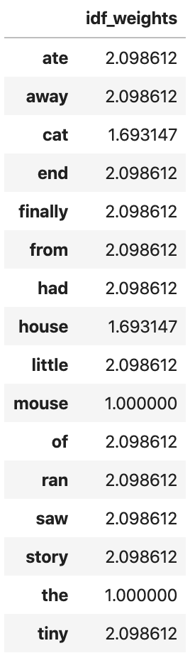

Note that the idf formula above differs from the standard textbook notation that defines the idf as idf(t) = log [ n / (df(t) + 1) ]) where n is the total number of documents in the document set and df(t) is the document frequency of t; the document frequency is the number of documents in the document set that contain the term t.

If smooth_idf=True (the default), the constant “1” is added to the numerator and denominator of the idf as if an extra document was seen containing every term in the collection exactly once, which prevents zero divisions: idf(d, t) = log [ (1 + n) / (1 + df(d, t)) ] + 1.

For example, the term cat appears in two documents and we have 5 documents. In other words, n=5 and df('cat') = 2. Thefore, inverse-document frequency for this word is:

 
np.log( (1+5)/(1+2)) + 1
#1.6931471805599454

Notice that the words ‘mouse’ and ‘the’ have the lowest IDF values. This is expected as these words appear in each and every document in our collection. The lower the IDF value of a word, the less unique it is to any particular document.

Once you have the IDF values, you can now compute the tf-idf scores for any document or set of documents. Let’s compute tf-idf scores for the 5 documents in our collection.

 
# count matrix
count_vector=cv.transform(docs)
 
# tf-idf scores
tf_idf_vector=tfidf_transformer.transform(count_vector)

The first line above, gets the word counts for the documents in a sparse matrix form. We could have actually used word_count_vector from above. However, in practice, you may be computing tf-idf scores on a set of new unseen documents. When you do that, you will first have to do cv.transform(your_new_docs) to generate the matrix of word counts.

Then, by invoking tfidf_transformer.transform(count_vector) you will finally be computing the tf-idf scores for your docs. Internally this is computing the tf * idf multiplication where your term frequency is weighted by its IDF values.

Now, let’s print the tf-idf values of the first document to see, by placing the tf-idf scores from the first document into a pandas data frame and sorting it in descending order of scores.

 
#get tfidf vector for first document
first_document_vector=tf_idf_vector[0]
 
#print the scores
df = pd.DataFrame(first_document_vector.T.todense(), index=tokens, columns=["tf-idf"])
df.sort_values(by=["tf-idf"],ascending=False)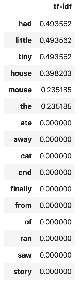

Notice that only certain words have scores because they only appear in the first document. The first document is “the house had a tiny little mouse” all the words in this document have a tf-idf score and everything else show up as zeroes. Notice that the word “a” is missing from this list. This is possibly due to internal pre-processing of CountVectorizer where it removes single characters. Note that the more common the word across documents, the lower its score and the more unique a word is to our first document (e.g. ‘had’ and ‘tiny’) the higher the score.

We can repeat the same process for all other documents.

Tfidfvectorizer Usage

This is another way of computing TF-IDF weights for terms in the document.

With Tfidfvectorizer you compute the word counts, idf and tf-idf values all at once. It’s really simple.

 
from sklearn.feature_extraction.text import TfidfVectorizer 
 
# settings that you use for count vectorizer will go here
tfidf_vectorizer=TfidfVectorizer(use_idf=True)
 
# just send in all your docs here
tfidf_vectorizer_vectors=tfidf_vectorizer.fit_transform(docs)

# get the first vector out (for the first document)
first_vector_tfidfvectorizer=tfidf_vectorizer_vectors[0]
 
# place tf-idf values in a pandas data frame
df = pd.DataFrame(first_vector_tfidfvectorizer.T.todense(), index=tfidf_vectorizer.get_feature_names(), columns=["tf_idf"])
df.sort_values(by=["tf_idf"],ascending=False)

Here’s another way to do it by calling fit and transform separately and you’ll end up with the same results.

 
tfidf_vectorizer=TfidfVectorizer(use_idf=True)
 
# just send in all your docs here
fitted_vectorizer=tfidf_vectorizer.fit(docs)
tfidf_vectorizer_vectors=fitted_vectorizer.transform(docs)