Written by
MMA
on
4 mins to read.
on
4 mins to read.
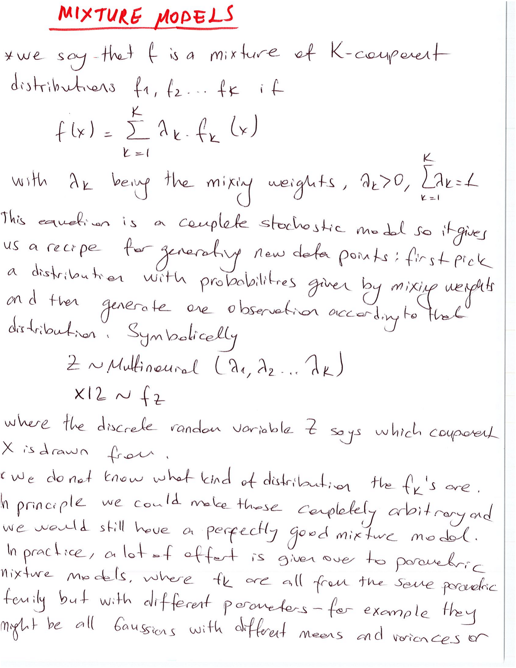
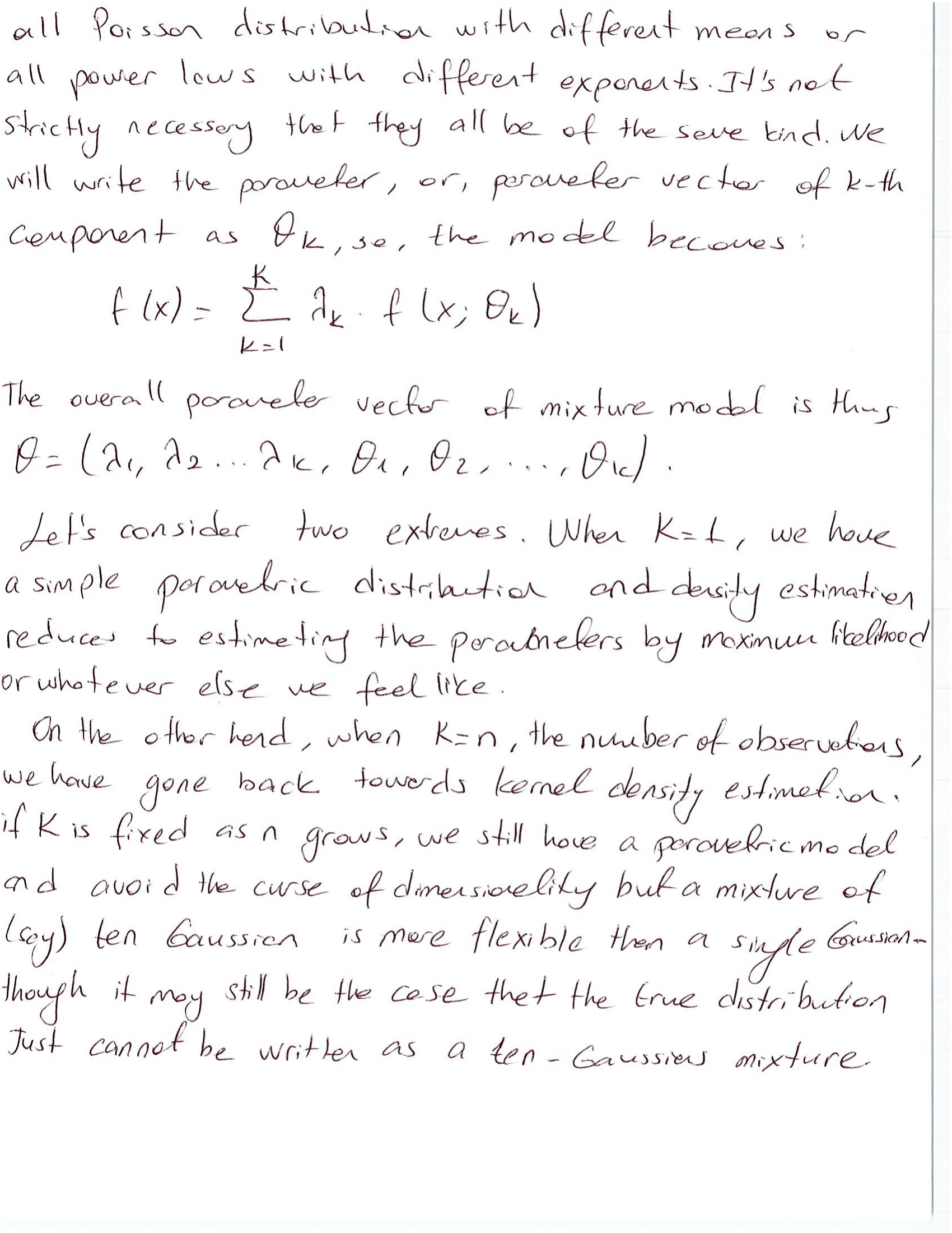
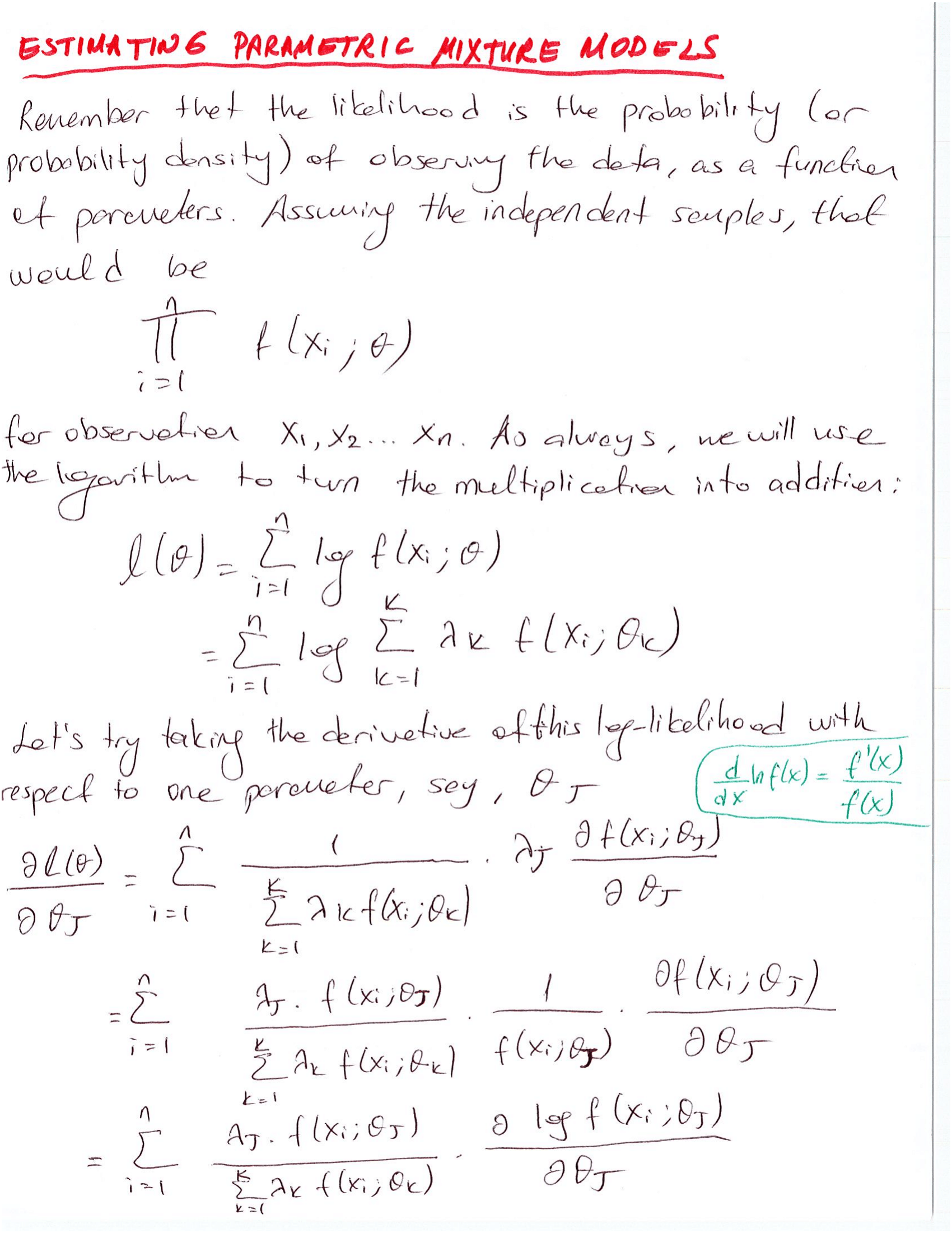
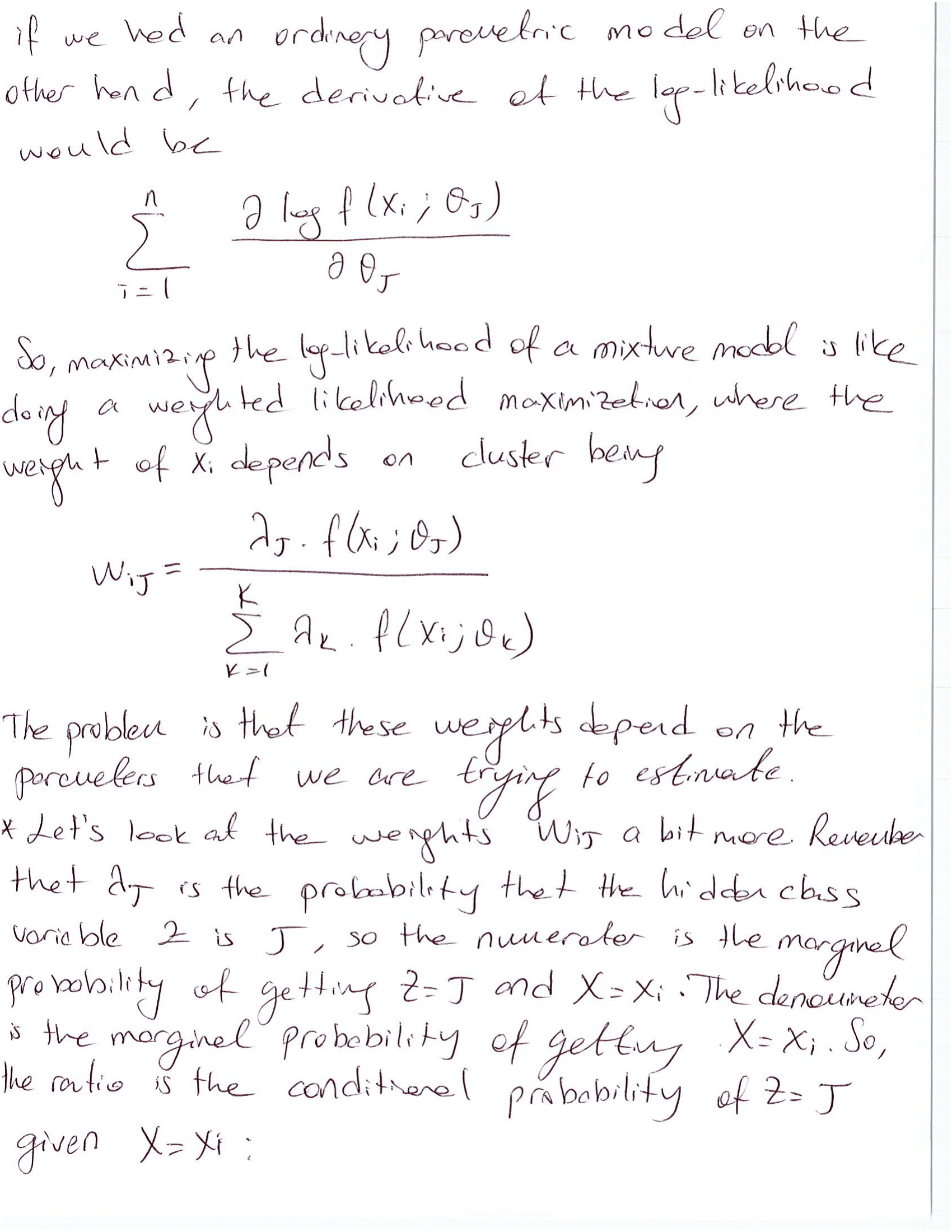
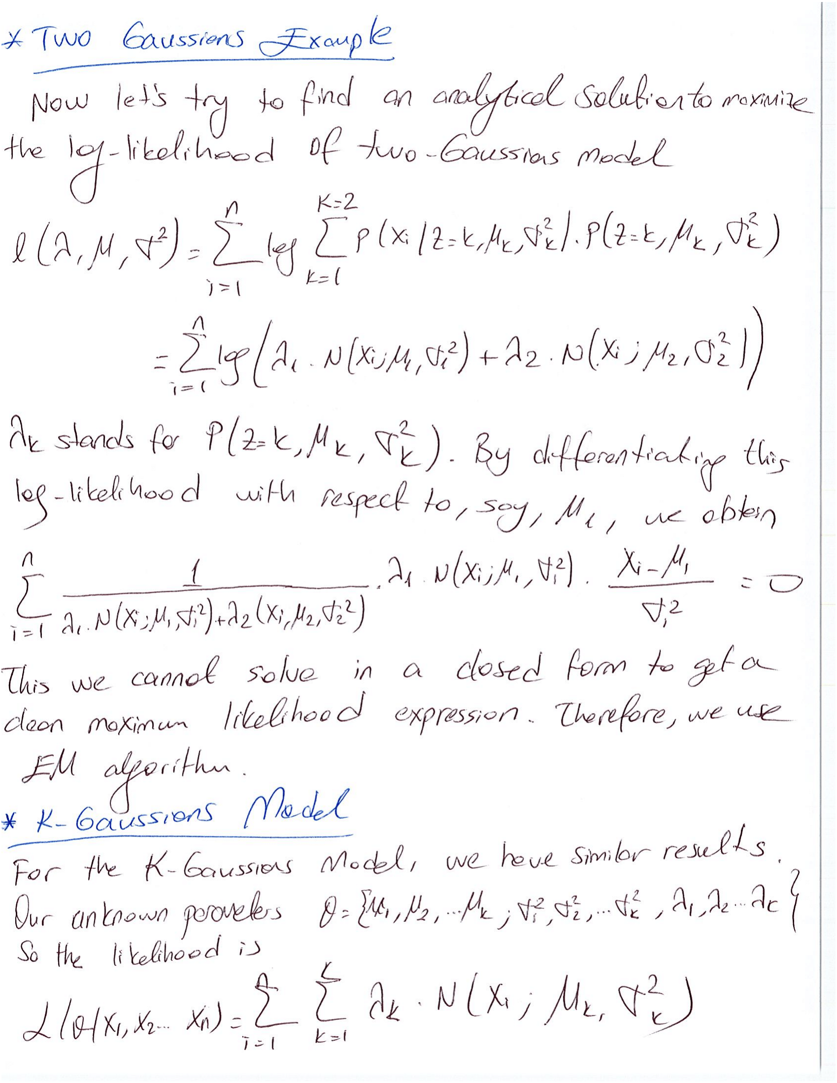
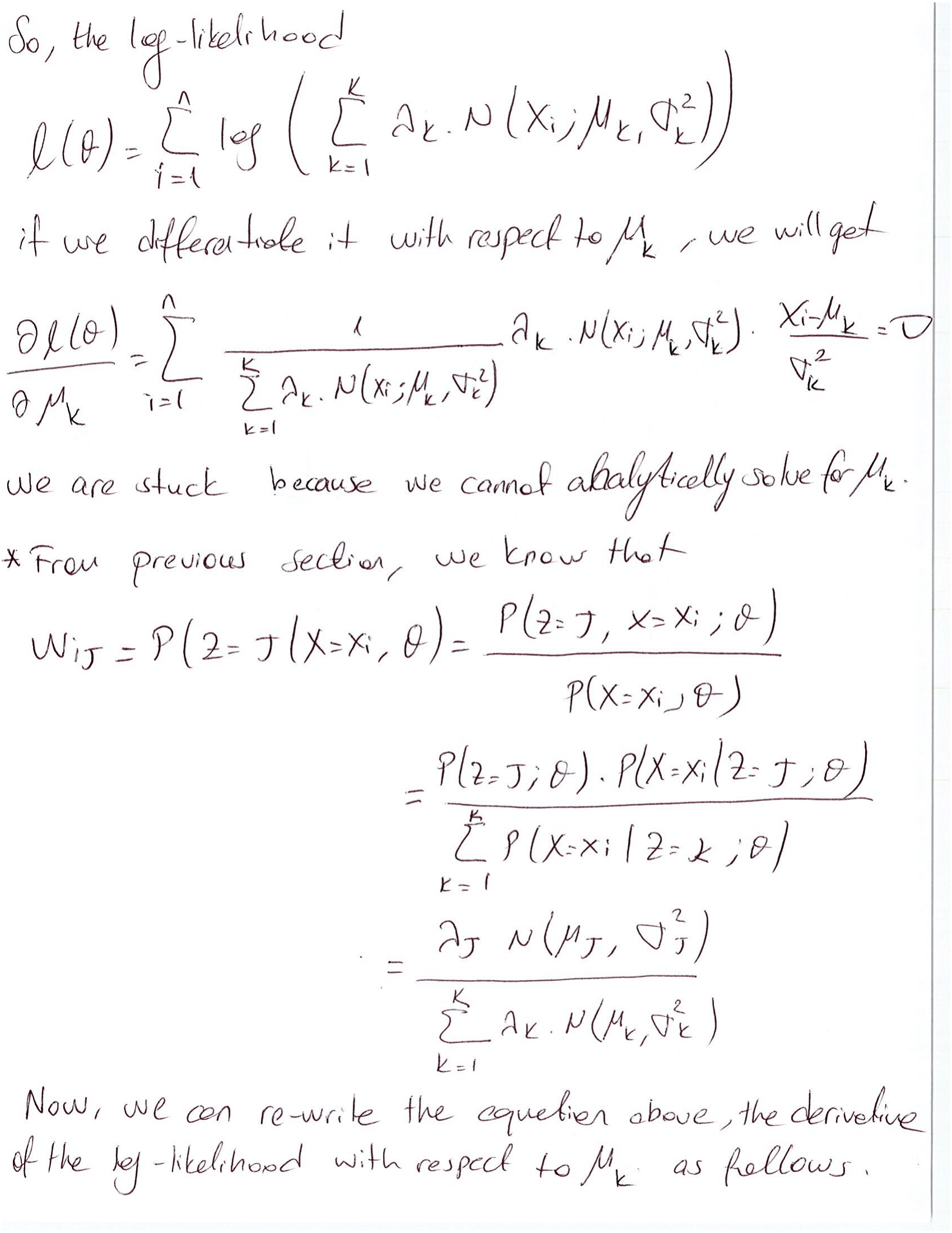
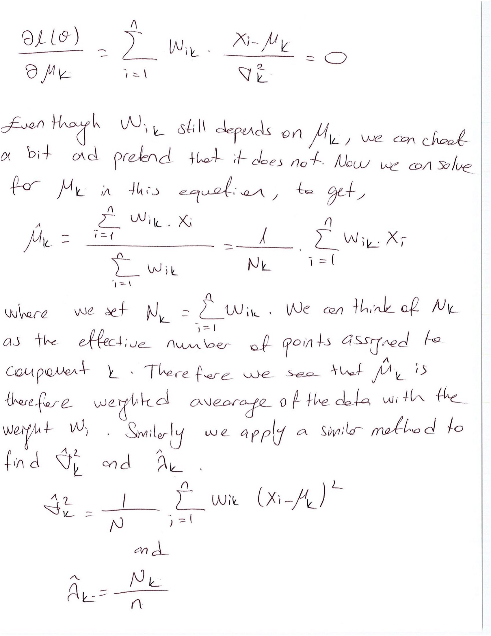
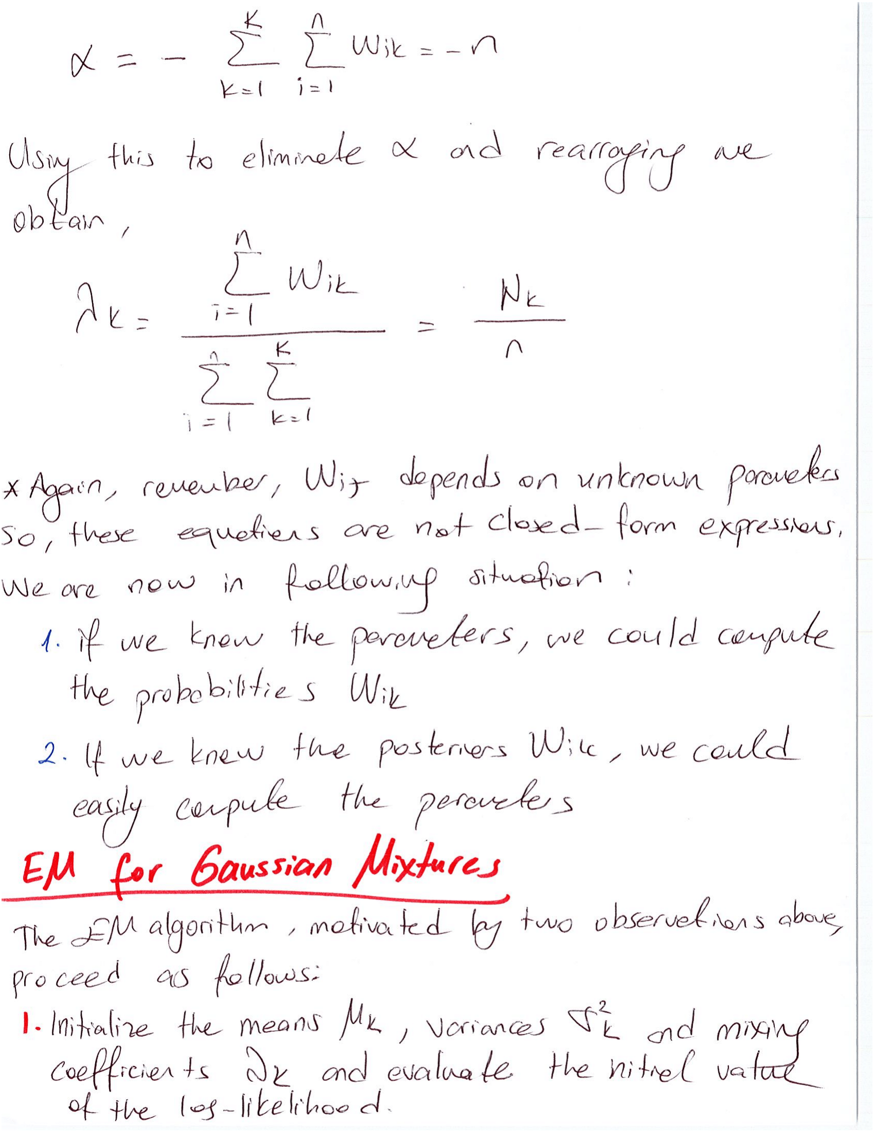
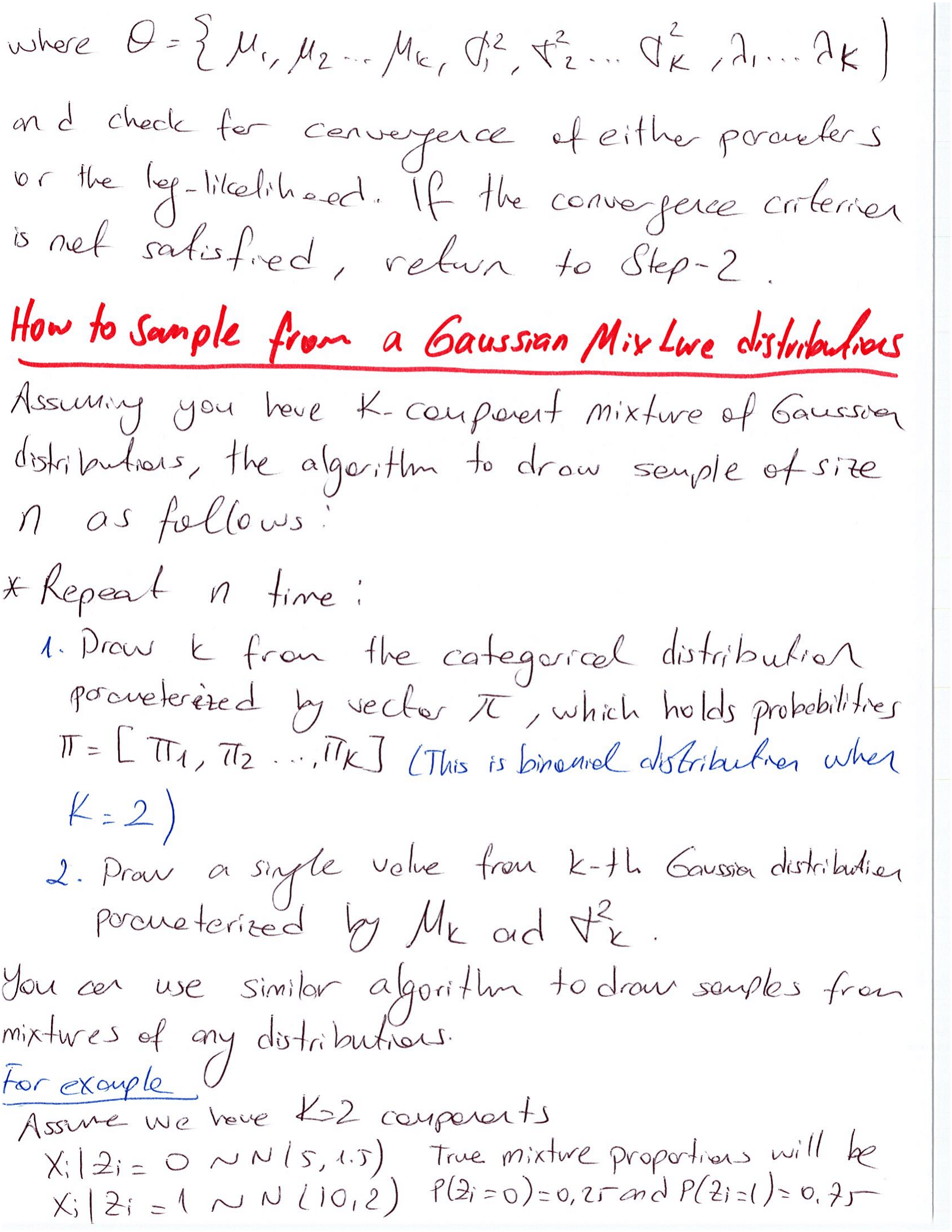
Gaussian Mixture Models in theoretical details
NOTE: This blog post consists of images. It might take a while to load in your browser!


import numpy as np
import seaborn as sns
import matplotlib.pyplot as plt
%matplotlib inline

mu = [5, 10]
sigma = [1.5, 2]
p_i = [0.25, 0.75]
n = 10000

x = []
z = []
for i in range(n):
    #We first choose which distribution to use, from these two Gaussians
    #so we have two options: 0 means the first Gaussian (N(5, 1.5)) and 1 means the second Gaussian (N(10, 2))
    z_i = np.random.binomial(1, 0.75)
    z.append(z_i)
    #[1, 0, 1, 1, 1, 0 ,0 ,1 ,0, ....., 1, 0] #Bernoulli
    x_i = np.random.normal(mu[z_i], sigma[z_i])
    x.append(x_i)

def univariate_normal(x, mean, variance):
    """pdf of the univariate normal distribution."""
    return ((1. / np.sqrt(2 * np.pi * variance)) *
            np.exp(-(x - mean)**2 / (2 * variance)))

a = np.arange(0, 18, 0.01)
y = p_i[0] * univariate_normal(a, mean=mu[0], variance=1.5**2) + p_i[1] * univariate_normal(a, mean=mu[1], variance=4)

fig, ax = plt.subplots(figsize=(8, 4))

ax.hist(x, bins='auto', density=True)
ax.plot(a, y)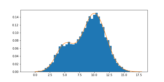
Three Gaussians Mixture distribution
import numpy as np
import matplotlib.pyplot as plt
%matplotlib inline

mu = [0, 10, 3]
sigma = [1, 1, 1]
p_i = [0.3, 0.5, 0.2]
n = 10000

x = []
for i in range(n):
    #When k is bigger than 2 and n is 1, Multinomial distribution is
    #the categorical distribution (multinoulli distribution).
    z_i = np.argmax(np.random.multinomial(1, p_i))
    x_i = np.random.normal(mu[z_i], sigma[z_i])
    x.append(x_i)

def univariate_normal(x, mean, variance):
    """pdf of the univariate normal distribution."""
    return ((1. / np.sqrt(2 * np.pi * variance)) *
            np.exp(-(x - mean)**2 / (2 * variance)))

a = np.arange(-7, 18, 0.01)
y = p_i[0] * univariate_normal(a, mean=mu[0], variance=sigma[0]**2) + p_i[1] * univariate_normal(a, mean=mu[1], variance=sigma[0]**2)+ p_i[2] * univariate_normal(a, mean=mu[2], variance=sigma[0]**2)

fig, ax = plt.subplots(figsize=(8, 4))

ax.hist(x, bins=100, density=True)
ax.plot(a, y)
