on
6 mins to read.
Poisson Regression in Tensorflow
In most of the classification problems, we have binary response variable. Now, let’s assume that we can only take non-negative integer values, i.e., 0, 1, 2,….Although it is very similar to classification, as we have integer values, there is no fixed upper bound and the variable is ordinal, so that the distance between 1 and 2 and 1 and 2 are not the same as we have in categorical data, e.g., one-hot encoded class labels.
This type of data, called count data, can be generated through a process where number of occurences of an event is counted. If the interval where we count occurences is fixed, then the process is called Poisson process and the data can be modelled using the Poisson distribution.
In this post, we will perform a Poisson regression with Tensorflow. Although Tensorflow is not primarily designed for traditional modeling tasks such as Poisson regression, we still can benefit from the flexibility of Tensorflow.
Poisson Formula
Suppose we conduct a Poisson experiment in which the average number of successes within a given region is $\lambda$. The Poisson probability is then given by:
\[P(y, \lambda) = \frac{e^{-\lambda}\lambda ^{y}}{y!},\,\,\,\,\ \lambda > 0\,\,\,\,\, \text{and}\,\,\,\,\ y=0,1,2,3,....\]where y is the actual number of successes that result from the experiment and only parameter $\lambda$ represent both the mean and the variance of the distribution.
\[E(y) = Var(y) = \lambda\]Poisson Regression Model
In Poisson regression, we suppose that the Poisson incidence rate $\lambda$ is determined by a set of $m$ variables. The expression relating these quantities is given by:
\[\log (\lambda_{i}) = \beta^{T} \cdot \mathbf{x}^{(i)}\]In addition to distribution assumption and independence between observations, we will now assume that:
\[E[y_{i} \mid \mathbf{x}^{(i)}] = \lambda_{i} = exp(\beta^{T} \cdot \mathbf{x}^{(i)})\]that is the mean of $y$ is conditional on X and can vary by individual or observation. Specific form of the link function is somewhat arbitrary but ensures that $\lambda_{i} > 0$. Here, $X_{i}$ is a n-dimensional predictor matrix and $\beta$ is a m-dimensional unknown coefficients. The exponential function (which corresponds to the log link function) is the classical one used in Poisson Regression, which makes sense since it brings the range from $(-\infty, \infty)$ to $(0,\infty)$ comparing it with sigmoid activation function in Bernoulli case.
The negative likelihood function of $\beta$ can be written then:
\[\begin{split} \mathcal{L} &= -log \left[\prod_{i=1}^{n}\frac{e^{-\lambda_{i}}\lambda_{i} ^{y_{i}}}{y_{i}!} \right]\\ &= -\sum_{i=1}^{n} y_{i} \log (\lambda_{i}) + \sum_{i=1}^{n} \lambda_{i} + \sum_{i=1}^{n} \log (y_{i}!)\\ &= - \sum_{i=1}^{n}y_{i} \beta^{T} \cdot \mathbf{x}^{(i)} + \sum_{i=1}^{n} exp(\beta^{T} \cdot \mathbf{x}^{(i)}) + \sum_{i=1}^{n} \log (y_{i}!) \end{split}\]Then, maximum likelihood estimator for $\beta$ is:
\[\hat{\beta} = \frac{\partial \mathcal{L}}{\partial \beta} = \sum_{i=1}^{n} (y_{i} - exp(\beta^{T} \cdot \mathbf{x}^{(i)})) \mathbf{x}_{i}\]Setting this equation equal to zero does not admit a closed form solution for $\beta$. Hence, a numerical method must be used in order to obtain the estimate.
Poisson Regression in Tensorflow
#Load the libraries
import tensorflow as tf
import tensorflow as tf
import numpy as np
import pandas as pd
import statsmodels.api as sm
import statsmodels.formula.api as smf

def gen_data(N = 10000):
    data = np.random.uniform(-1, 1, (N, 3))
    data = sm.add_constant(data)
    data = pd.DataFrame(data, columns = ['intercept', 'Var1', 'Var2', 'Var3'])
    lam = np.exp(-2*data['intercept'] + data['Var1'] - 0.5*data['Var2'] + 0.3*data['Var3'] )
    resp = np.random.poisson(lam = lam)
    data['lam'] = lam
    data['response'] = resp
    return data

dtrain = gen_data()
dtrain.drop('lam', axis=1)

X = tf.constant(dtrain[['intercept', 'Var1', 'Var2', 'Var3']].values, name = 'X', dtype=tf.float32)
# <tf.Tensor 'X:0' shape=(10000, 4) dtype=float32>

y = tf.constant(value = list(dtrain['response']), dtype = tf.float32, name='y', shape=(dtrain.shape[0], 1))
# <tf.Tensor 'y:0' shape=(10000, 1) dtype=float32>

parameters = tf.Variable(tf.zeros([4, 1])) #Initial Values
# <tf.Variable 'Variable:0' shape=(4, 1) dtype=float32_ref>

logits = tf.matmul(X, parameters, name="logits")
# <tf.Tensor 'logits:0' shape=(10000, 1) dtype=float32>

y_hat = tf.exp(logits)

# create the loss
loss = tf.reduce_mean(-y*tf.log(y_hat)+y_hat)
# last term can be avoided since it doesn't depend on y_pred
# however keeping it gives a nice lower bound to zero
# tf.lgamma computes the log of the absolute value of Gamma(x) element-wise

learning_rate = 0.001
optimizer = tf.train.AdamOptimizer(learning_rate=learning_rate)
training_op = optimizer.minimize(loss)

n_epochs = 10000

with tf.Session() as sess:
    tf.global_variables_initializer().run()
    for epoch in range(n_epochs):
        sess.run(training_op)
        if epoch % 100 == 0:
            print("Epoch", epoch, "Loss = ", loss.eval())
    best_parameters = parameters.eval()

print(best_parameters)
# [[-2.008499  ]
#  [ 0.9841952 ]
#  [-0.59924984]
#  [ 0.25809023]]
Comparison with the statsmodels package
To check the results, we repeat solving the same regression problem using the statsmodels library:
statsmodels.api
output = dtrain['response']
inputs = dtrain.drop('response', axis=1)
poisson_model = sm.GLM(output, inputs, family=sm.families.family.Poisson(link=sm.genmod.families.links.log)).fit()
poisson_model.summary()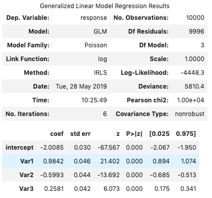
statsmodels.formula.api
#In statsmodels.formula.api, a constant is automatically added to your data and an intercept in fitted
# in statsmodels.api, you have to add a constant yourself. Try using add_constant from statsmodels.api
#https://stackoverflow.com/questions/30650257/ols-using-statsmodel-formula-api-versus-statsmodel-api
dtrain.drop('intercept', axis=1)
formula = "dtrain['resp'] ~ dtrain['Var1'] + dtrain['Var2'] + dtrain['Var3']"
poisson = smf.poisson(formula, data=dtrain).fit(method='bfgs')
poisson.summary()