Some Basic Activation Functions

Activation Functions

Activation functions help in achieving non-linearity in deep learning models. If we don’t use these non-linear activation functions, neural network would not be able to solve the complex real life problems like image, video, audio, voice and text processing, natural language processing etc. because our neural network would still be linear and linear models cannot solve real life complex problems. These activation functions are also called squashing functions as these functions squash the output under certain range. We will also see various advantages and disadvantages of different activation functions.

Sigmoid Function

Sigmoid function is one of the mostly-used and well-known activation functions. The function itself is defined as:

and its first-order derivative is given by

This turns out to be a convenient form for efficiently calculating gradients used in neural networks. If one keeps in memory the feed-forward activations of the sigmoid (logistic) function for a given layer, the gradients for that layer can be evaluated using simple multiplication and subtraction rather than performing any re-evaluating the sigmoid function, which requires extra exponentiation.

import numpy as np
import matplotlib
import matplotlib.pyplot as plt
%matplotlib inline

def sigmoid(z):
    return 1/ (1+np.exp(-z))

def sigmoid_derivation(z):
    return sigmoid(z)*(1-sigmoid(z))

z = np.linspace(-5, 5, 200)
plt.figure()
plt.style.use('seaborn-darkgrid')
plt.plot(z, sigmoid(z), "b-.", linewidth=2)
props = dict(facecolor='black', shrink=0.1)
plt.annotate('Saturating', xytext=(3.5, 0.7), xy=(5, 1), arrowprops=props, fontsize=14, ha="center")
plt.annotate('Saturating', xytext=(-3.5, 0.3), xy=(-5, 0), arrowprops=props, fontsize=14, ha="center")
plt.title("Sigmoid Activation Function", fontsize=14)
plt.savefig('sigmoid.png')

z = np.linspace(-5, 5, 200)
plt.figure()
plt.style.use('seaborn-darkgrid')
plt.plot(z, sigmoid_derivation(z), "b-.", linewidth=2)
props = dict(facecolor='black', shrink=0.1)
plt.annotate('Max Value', xytext=(0, 0.15), xy=(0, 0.25), arrowprops=props, fontsize=14, ha="center")
plt.title("Derivation of Sigmoid Function", fontsize=14)
plt.savefig('sigmoid_derivation.png')

The plot of sigmoid function and its derivative are shown as follows:

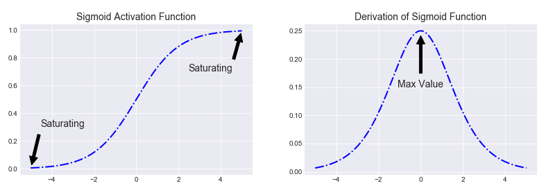
Sigmoid function is non-linear in nature. Combinations of this function are also non-linear. So, stacking layers is possible. Non-binary activations is also feasible because it will spit out intermediate activation values unlike step function. It has a smooth gradient too.

Figure shows that between x values -2 to 2, y values are very steep, which means that any small changes in the values of x in that region will cause values of y to change significantly. That means this function has a tendency to bring the y values to either end of the curve, which will make clear distinctions on prediction. The output of the activation function is always going to be in range $(0,1)$ compared to $(-\infty, \infty)$ of linear function. So we have our activations bound in a range. The activations will not blow up then. However, there are couple of problems with sigmoid function.

Towards either end of the sigmoid function, the y values tend to respond very less to changes in x. The gradient at that region is going to be small. It gives rise to a problem of “vanishing gradients” because derivative of sigmoid is always less than 0.25 for all inputs except 0. Sigmoid neurons will stop learning when they saturate. Gradient is small or has vanished and it cannot make significant change because of the extremely small value. The network refuses to learn further or is drastically slow depending on the case and until gradient/computation gets hit by floating point value limits. Because if one multiples a bunch of terms which are less than 1, the result will tend towards the zero. Hence gradients will vanish as going further away from the output layer. There are ways to work around this problem and sigmoid is still very popular in classification problems.

Hyperbolic Tangent Function

Another popular activation function is Hyperbolic Tangent function. Hyperbolic Tangent function, also known as tanh function, is a rescaled version of the sigmoid function. The function itself is defined as

and its derivative is given by

import numpy as np
import matplotlib
import matplotlib.pyplot as plt
%matplotlib inline

def tanh(z):
    return (np.exp(z)-np.exp(-z))/(np.exp(z)+np.exp(-z))

def tanh_derivation(z):
    return (1- tanh(z)**2)

z = np.linspace(-5, 5, 200)
plt.figure()
plt.style.use('seaborn-darkgrid')
plt.plot(z, tanh(z), "b-.", linewidth=2)
props = dict(facecolor='black', shrink=0.1)
plt.annotate('Saturating', xytext=(3.5, 0.7), xy=(5, 1), arrowprops=props, fontsize=14, ha="center")
plt.annotate('Saturating', xytext=(-3.5, 0.3), xy=(-5, 0), arrowprops=props, fontsize=14, ha="center")
plt.title("Hyperbolic Tangent Activation Function", fontsize=14)
plt.savefig('tanh.png')

z = np.linspace(-5, 5, 200)
plt.figure()
plt.style.use('seaborn-darkgrid')
plt.plot(z, tanh_derivation(z), "b-.", linewidth=2)
props = dict(facecolor='black', shrink=0.1)
plt.annotate('Max Value', xytext=(2.9, 0.8), xy=(0, 1), arrowprops=props, fontsize=14, ha="center")
plt.title("Derivation of Hyperbolic Tangent Function", fontsize=14)
plt.savefig('tanh_derivation.png')

The plot of hyperbolic tangent function and its derivative are shown as follows:

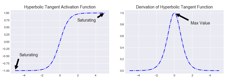
Similar to the derivative of the sigmoid function, the same caching trick can be used for layers that implement tanh activation function.

It has characteristics similar to sigmoid function. It is nonlinear in nature, so, we can stack layers. The tanh non-linearity squashes real numbers to range between $[-1,1]$ so one needs not to worry about activations blowing up. The gradient is stronger for tanh than sigmoid (derivatives are steeper). Deciding between the sigmoid or tanh will depend on your requirement of gradient strength. However, unlike the sigmoid neuron, the output of tanh function is zero-centered. Therefore, in practice the tanh non-linearity is always preferred to the sigmoid nonlinearity (source).

Like sigmoid function, tanh function also has the vanishing gradient problem because the derivative of the function is always less than 1 for all inputs except 0.

Instead of sigmoid function and tanh function because of all these problems associated with them, the most recent deep learning networks use rectified linear units (ReLUs) for the hidden layers which might be a solution for vanishing gradient problem.

Rectified Linear Unit (ReLU)

ReLU is a piecewise non-linear function that corresponds to:

Another way of writing the ReLU function is like so:

where $x$ is the input to a neuron. In other words, when the input is smaller than zero, the function will output zero. Else, the function will mimic the identity function. So, the range of ReLU is between $0$ to $\infty$.

ReLU is less computationally expensive than tanh and sigmoid neurons due to its linear, non-saturating form and involving simpler mathematical operations. It’s very fast to compute because its derivative is easy to handle. When the input is greater or equal to zero, the output is simply the input, and hence the derivative is equal to one. The function is not differentiable at zero, though. In other words, when the input is smaller than zero, the function will output zero. Else, the function will mimic the identity function. It is linear in positive axis. Therefore, the derivative of ReLU is:

Note that derivative of ReLU function at $x=0$ does not exist.

A function is only differentiable if the derivative exists for each value in the function’s domain (for instance, at each point). One criterion for the derivative to exist at a given point is continuity at that point. However, the continuity is not sufficient for the derivative to exist. For the derivative to exist, we require the left-hand and the right-hand limit to exist and be equal.

General definition of the derivative of a continuous function $f(x)$ is given by:

where $\lim_{h \rightarrow 0}$ means “as the change in h becomes infinitely small (for instance h approaches to zero)”.

Let’s get back to ReLU function. If we substitute the ReLU equation into the limit definition of derivative above:

Next, let us compute the left- and right-side limits. Starting from the left side, where $\Delta x$ is an infinitely small, negative number, we get,

And for the right-hand limit, where $\Delta x$ is an infinitely small, positive number, we get:

The left- and right-hand limits are not equal at $x=0$; hence, the derivative of ReLU function at $x=0$ is not defined.

import numpy as np
import matplotlib
import matplotlib.pyplot as plt
%matplotlib inline

def relu(z):
    return np.maximum(0, z)

def derivative_relu(z):
    return (z >= 0).astype(z.dtype)

z = np.linspace(-5, 5, 200)

plt.figure()
plt.plot(z, derivative_relu(z), "g-.", linewidth=2, label="ReLU Derivation")
plt.grid(True)
plt.legend(loc='upper left', fontsize=12)
plt.title("Derivative of ReLU Activation Function", fontsize=14)
plt.savefig('relu_derivative.png')

plt.figure()
plt.plot(z, relu(z), "b-.", linewidth=2, label="ReLU")
plt.grid(True)
plt.legend(loc='upper left', fontsize=12)
plt.title("ReLU Activation Function", fontsize=14)
plt.savefig('relu.png')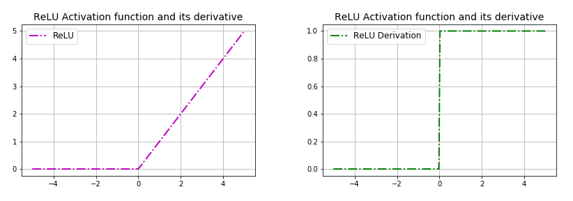

ReLU is non-linear in nature and combinations of ReLU functions are also non-linear. In fact, it is a good approximator. Any function can be approximated with combinations of ReLUs. This means that we can stack layers. It is not bounded though. The range of ReLU is $[0,\infty)$. It does not saturate but it is possible that activations can blow up.

However there is a huge advantage with ReLU function. The rectifier activation function introduces sparsity effect on the network. Using a sigmoid or hyperbolic tangent will because almost all neurons to fire in an analog way. That means almost all activations will be processed to describe the output of a network. In other words the activation is dense. This is costly. We would ideally want a few neurons in the network to not activate and thereby making the activations sparse and efficient. ReLU gives us this benefit. Sparsity results in concise models that often have better predictive power and less overfitting/noise. A sparse network is faster than a dense network, as there are fewer things to compute.

Because of the horizontal line in ReLU (for negative X), unfortunately, ReLUs can be fragile during training and can “die” irreversibly, which means vanishing. For activations in that region of ReLU, gradient will be 0 from that point on because the weights will not get adjusted during descent. That means, those neurons, which go into that state, will stop responding to variations in error/ input. This is called dying ReLU problem. This problem can cause several neurons to just die and not respond making a substantial part of the network passive.

So, for the ReLU activator, if weights and bias go all negative for example, the activation function output will be on the negative axis (which is just $y = 0$) and from then onwards, there is no way it can adjust itself back to life (non-zero) unless there is an external factor to change the outputs of the layer to something else than negative. Even though there are some extremely useful properties of gradients dying off for the idea of “sparsity”, Died ReLU is a problem during training process but is an advantage on a trained fit. We wanted some neurons to not respond and just stay dead, making the activations sparse (at the same time, the network should be accurate, meaning, the right ones should die) but during the training process if the wrong ones die, those do not recover until externally fixed. Dying ReLU is a problem because it can prevent the network from converging or building accuracy during the training process.

Implementing ReLU in TensorFlow is trivial, just specify the activation function when building each layer using tf.nn.relu.

ReLU Variants

Leaky ReLU & Parametric ReLU (PReLU)

A variant was introduced for ReLU to mitigate this issue by simply making the horizontal line into non-horizontal component. The main idea is to let the gradient be non-zero and recover during training eventually and keep learning. Leaky ReLUs are one attempt to fix the dying ReLU problem. Leaky units are the ones that have a very small gradient instead of a zero gradient when the input is negative, giving the chance for the network to continue its learning.

The hyperparameter $\alpha$ defines how much the function “leaks”: it is the slope of the function for $x <0$ and is typically set to $0.01$.

import numpy as np
import matplotlib
import matplotlib.pyplot as plt
%matplotlib inline


def leaky_relu(z, alpha=0.01):
    return np.maximum(alpha*z, z)

z = np.linspace(-5, 5, 200)
plt.plot(z, leaky_relu(z, 0.05), "b-", linewidth=2)
plt.plot([-5, 5], [0, 0], 'k-')
plt.plot([0, 0], [-0.5, 4.2], 'k-')
plt.grid(True)
props = dict(facecolor='black', shrink=0.1)
plt.annotate('Leak', xytext=(-3.5, 0.5), xy=(-5, -0.2), arrowprops=props, fontsize=14, ha="center")
plt.title("Leaky ReLU activation function", fontsize=14)
plt.axis([-5, 5, -0.5, 4.2])

plt.savefig("leaky_relu_plot")
plt.show()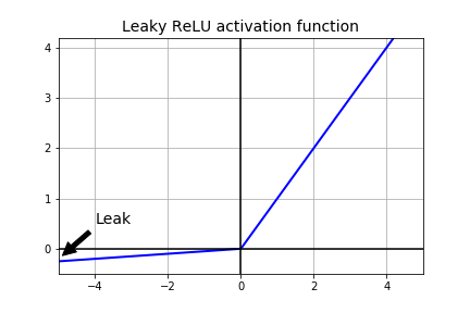

Similar to ReLU, because the output of Leaky ReLU isn’t bounded between 0 and 1 or −1 and 1 like hyperbolic tangent/sigmoid neurons are, the activations (values in the neurons in the network, not the gradients) can in fact explode with extremely deep neural networks like recurrent neural networks. During training, the whole network becomes fragile and unstable in that, if you update weights in the wrong direction, even the slightest, the activations can blow up. Finally, even though the ReLU derivatives are either 0 or 1, our overall derivative expression contains the weights multiplied in. Even though ReLU is much more resistant to vanishing gradient problem, since the weights are generally initialized to be < 1, this could contribute to vanishing gradients. However, overall, it’s not a black and white problem. ReLUs still face the vanishing gradient problem, it’s just that researchers often face it to a lesser degree.

Another type of ReLU that has been introduced is Parametric ReLU (PReLU). Here, instead of having $\alpha$ predetermined slope like $0.01$, $\alpha$ is to be learned during training. It is reported that PReLU strongly outperform ReLU on large image datasets but on smaller datasets, it runs the risk of overfitting the training set.

Implementing Leaky ReLU in TensorFlow is trivial, just specify the activation function when building each layer using tf.nn.leaky_relu.

Similarly, implementing Parametric ReLU in TensorFlow is trivial, just specify the activation function when building each layer using tf.keras.layers.PReLU.

NOTE: The ideas behind the LReLU and PReLU are similar. However, Leaky ReLUs have $\alpha$ as a hyperparameter and Parametric ReLUs have $\alpha$ as a parameter.

Exponential Linear (ELU, SELU)

Similar to leaky ReLU, ELU has a small slope for negative values. Instead of a straight line, it uses a log curve. ELU outperformed all the ReLU variants in the original paper’s experiments: training time was reduced and the neural network performed better on the test set. ELU is given by:

import numpy as np
import matplotlib
import matplotlib.pyplot as plt
%matplotlib inline

def elu(z, alpha=1):
    return np.where(z < 0, alpha * (np.exp(z) - 1), z)

z = np.linspace(-5, 5, 200)
plt.plot(z, elu(z), "b-", linewidth=2)
plt.plot([-5, 5], [0, 0], 'k-')
plt.plot([-5, 5], [-1, -1], 'k--')
plt.plot([0, 0], [-2.2, 3.2], 'k-')
plt.grid(True)
plt.title(r"ELU activation function ($\alpha=1$)", fontsize=14)
plt.axis([-5, 5, -2.2, 3.2])

plt.savefig("elu_plot")
plt.show()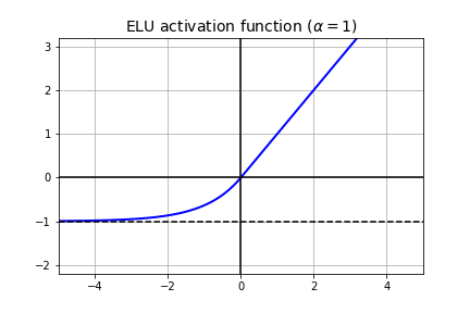

The main drawback of the ELU activation function is that it is slower to compute than the ReLU and its variants due to the use of the exponential function but during training this is compensated by the faster convergence rate. However, at test time, an ELU network will be slower than a ReLU network.

Implementing ELU in TensorFlow is trivial, just specify the activation function when building each layer using tf.nn.elu.

Scaled exponential linear unit (SELU) has also been proposed in the literature. SELU is some kind of ELU but with a little twist. $\alpha$ and $\lambda$ are two pre-defined constants, meaning we don’t backpropagate through them and they are not hyperparameters to make decisions about. $\alpha$ and $\lambda$ are derived from the inputs. $\lambda$ is called as a scale parameter. Essentially, SELU is scale * elu(x, alpha).

SELU can’t make it work alone. Thus, a custom weight initialization technique is being used. It is to be used together with the initialization “lecun_normal”, which it draws samples from a truncated normal distribution centered on $0$ with stddev <- sqrt(1 / fan_in) where fan_in is the number of input units in the weight tensor.

For standard scaled inputs (mean 0, stddev 1), the values are $\alpha \approx 1.6732$, $\lambda \approx 1.0507$. Let’s plot and see what it looks like for these values.

import numpy as np
import matplotlib
import matplotlib.pyplot as plt
%matplotlib inline

def selu(z, alpha=1.6732632423543772848170429916717, lamb=1.0507009873554804934193349852946):
    return np.where(z < 0, lamb * alpha * (np.exp(z) - 1), z)

z = np.linspace(-5, 5, 200)
plt.plot(z, selu(z), "b-", linewidth=2)
plt.plot([-5, 5], [0, 0], 'k-')
plt.plot([-5, 5], [-1, -1], 'k--')
plt.plot([0, 0], [-2.2, 3.2], 'k-')
plt.grid(True)
plt.title(r"SELU activation function ($\alpha \approx 1.6732$ and $\lambda \approx 1.0507$)", fontsize=14)
plt.axis([-5, 5, -2.2, 3.2])

plt.savefig("selu_plot")
plt.show()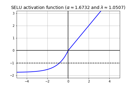

Implementing SELU in TensorFlow is trivial, just specify the activation function when building each layer using tf.nn.selu.

Concatenated ReLU (CReLU)

It concatenates a ReLU which selects only the positive part of the activation with a ReLU which selects only the negative part of the activation. In other words, for positive $x$ it produces $[x, 0]$, and for negative $x$ it produces $[0, x]$. Note that it has two outputs, as a result this non-linearity doubles the depth of the activations.

Implementing CReLU in TensorFlow is trivial, just specify the activation function when building each layer using tf.nn.crelu.

ReLU-6

You may run into ReLU-6 in some libraries, which is ReLU capped at 6.

import numpy as np
import matplotlib
import matplotlib.pyplot as plt
%matplotlib inline

def relu_6(z):
    return np.where(z < 6, np.maximum(0, z), 6) 

z = np.linspace(-5, 20, 200)
plt.figure()
plt.style.use('seaborn-darkgrid')
plt.plot(z, relu(z), "b-.", linewidth=2)
plt.grid(True)
plt.legend(loc='upper left', fontsize=12)
plt.title("ReLU-6 Activation Function", fontsize=14)
plt.savefig('relu-6.png')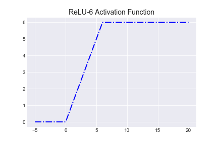

It was first used in this paper for CIFAR-10, and 6 is an arbitrary choice that worked well. According to the authors, the upper bound encouraged their model to learn sparse features earlier.

Implementing ReLU-6 in TensorFlow is trivial, just specify the activation function when building each layer using tf.nn.relu6.

REFERENCES

1. Paul J. Werbos. Backpropagation through time: what it does and how to do it. Proceedings of the IEEE, 78(10): 1550 – 1560, 1990.

2. https://www.utc.fr/~bordesan/dokuwiki/_media/en/glorot10nipsworkshop.pdf

3. https://arxiv.org/abs/1511.07289

4. https://arxiv.org/abs/1706.02515

5. https://arxiv.org/abs/1603.05201

6. https://ayearofai.com/rohan-4-the-vanishing-gradient-problem-ec68f76ffb9b