Logistic Regression in Tensorflow

Linear regression assumes linear relationships between variables. This assumption is usually violated when the dependent variable is categorical. The logistic regression equation expresses the multiple linear regression equation in logarithmic terms and thereby overcomes the problem of violating the linearity assumption.

Logistic Regression is one of the methods that have been used for classification problem. It is commonly used to estimate the probability that an instance belongs to a particular class (e.g., what is the probability that this email is spam?). If the estimated probability is greater than 50\%, then the model predicts that the instance belongs to that class (called the positive class, labeled as “1”) or else it predicts that it does not (i.e., it belongs to the negative class, labeled as “0”). This makes it a binary classifier.

Estimating probabilities

A Logistic Regression model computes a weighted sum of input features (plus a bias term), but instead of outputting the result directly like Linear Regression model does, it outputs logistic of this result.

So we have a dataset $\mathbf{X}$ consisting of $m$ datapoints and $n$ features. And there is a class variable $y$ a vector of length $m$ which can have two values $1$ for positive class or $0$ for negative class. Actually $y^{(i)}$ follows a Bernoulli distribution for binary classification. Now logistic regression says that the probability that class variable value $y^{(i)}=1, i=1, 2, \cdots, m$ can be modelled as follows:

\[h_{\theta} ( \mathbf{x}^{(i)} ) = E \left[y^{(i)} \mid \mathbf{x}^{(i)}\right] = P(y^{(i)}=1 \mid \mathbf{x}^{(i)}, \theta) = 0 \times P(y^{(i)}=0 \mid \mathbf{x}^{(i)}, \theta) + 1 \times P(y^{(i)}=1 \mid \mathbf{x}^{(i)}, \theta) = \sigma \left( \theta^{T} \cdot \mathbf{x}^{(i)} \right)\]

where $\sigma$ represents sigmoid (logistic) function. But why?

The reason comes from generalized linear models. Given that $y$ is binary-valued, it therefore seems natural to choose Bernoulli family of distributions to model the conditional distribution of $y$ given $x$. In the formulation of Bernoulli distribution as an exponential family distribution, we have $p = \frac{1}{1+ e^{-\eta}}$. Furthermore, note that if $y \mid x; \theta \sim Bernoulli(p)$, then $E \left[y \mid x\right] = p$.

\[h_{\theta} ( \mathbf{x}^{(i)} ) = E \left[y^{(i)} \mid \mathbf{x}^{(i)}\right] = P(y^{(i)}=1 \mid \mathbf{x}^{(i)}, \theta) = \frac{1}{1+ e^{-\eta}} = \frac{1}{1+ e^{-\theta^{T} \cdot \mathbf{x}^{(i)}}}\]

where $\eta = \theta^{T} \cdot \mathbf{x}^{(i)}$ can be written as $\theta_{0} + \theta_{1} x_{1}^{(i)} + \theta_{2}x_{2}^{(i)} + \cdots + \theta_{n} x_{n}^{(i)}$.

Here, fitting the model $\theta^{T} \cdot \mathbf{x}^{(i)}$ does not ensure that the probability $p$ will end up in 0 and 1, as a probability must. Because it is unbounded. The linear combination goes from negative infinity to positive infinity. Therefore, we model $p$ by applying a logistic response or inverse logistic function ($\sigma$) to the predictors. This transform ensures that probability lies between 0 and 1.

Sigmoid Function

The logistic - also called the logit, noted $\sigma(\cdot)$ - is a sigmoid function (i.e., S-shaped) that outputs a number between 0 and 1. It is defined as the following:

\[\sigma(t) = \dfrac{1}{1+exp(-t)}\]

Therefore, we can re-write Logistic Regression model equation as follows:

\[\begin{align} P(y^{(i)}=1 \mid \mathbf{x}^{(i)}, \theta)= \sigma\left( \theta^{T} \cdot \mathbf{x}^{(i)} \right) &= \dfrac{1}{1+exp(-\theta^{T} \cdot \mathbf{x}^{(i)})}\\ &= \dfrac{1}{1+exp(-(\theta_{0} + \theta_{1} x_{1}^{(i)} + \theta_{2}x_{2}^{(i)} + \cdots + \theta_{n} x_{n}^{(i)}))} \\ &= \dfrac{exp(\theta_{0} + \theta_{1} x_{1}^{(i)} + \theta_{2}x_{2}^{(i)} + \cdots + \theta_{n} x_{n}^{(i)})}{1+exp(\theta_{0} + \theta_{1} x_{1}^{(i)} + \theta_{2}x_{2}^{(i)} + \cdots + \theta_{n} x_{n}^{(i)})} \end{align}\]

where $n$ is the number of features in the data, $x_{i}$ is the $i$th feature value and $\theta_{j}$ is the $j$th model parameter (including the bias term $\theta_{0}$).

Once the Logistic Regression model has estimated the probability $\hat{p}^{(i)} = h_{\theta} ( \mathbf{x}^{(i)} )$ that an instance $\mathbf{x}^{(i)}$ belongs to the positive class, it can make its prediction $\hat{y}^{(i)}$ easily. In order to predict which class a data belongs, a threshold can be set. Based upon this threshold, the obtained estimated probability is classified into classes:

\[\hat{y}^{(i)} = \left\{ \begin{array}{ll} 0 & \mbox{if $\hat{p}^{(i)} < 0.5$};\\ 1 & \mbox{if $\hat{p}^{(i)} \geq 0.5$}.\end{array} \right.\]

Notice that $\sigma (t) < 0.5$ when $t<0$ and $\sigma (t) \geq 0.5$ when $t \geq 0$, so, a Logistic Regression model predicts 1 if $\theta^{T} \cdot \mathbf{x}^{(i)}$ is positive, and 0 if it is negative.

Cost Function

Cost function which has been used for linear can not be used for logistic regression. Linear regression uses mean squared error as its cost function. If this is used for logistic regression, then it will be a non-convex function of parameters ($\theta$). Gradient descent will converge into global minimum only if the function is convex.

This strange outcome is due to the fact that in logistic regression we have the sigmoid function around, which is non-linear (i.e. not a line). The gradient descent algorithm might get stuck in a local minimum point. That’s why we still need a neat convex function as we did for linear regression: a bowl-shaped function that eases the gradient descent function’s work to converge to the optimal minimum point.

Instead of Mean Squared Error, we use a cost function called Cross-Entropy, also known as Log Loss. Cross-entropy loss can be divided into two separate cost functions: one for $y^{(i)}=1$ and one for $y^{(i)}=0$ for $i$th observation.

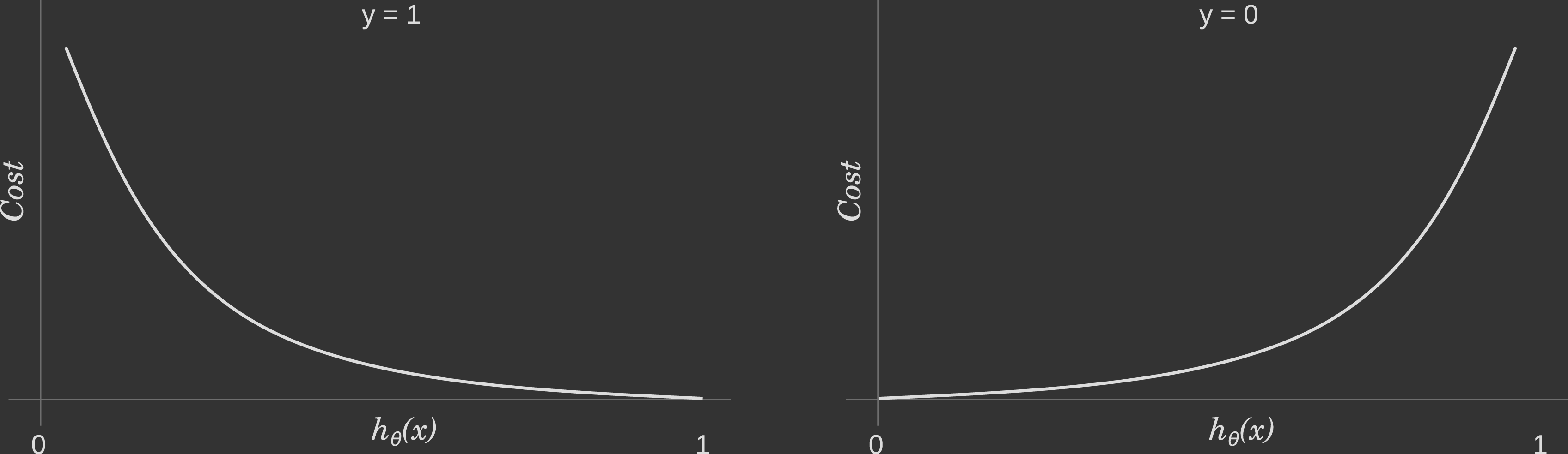
\[\mathrm{Cost}(h_{\theta}(\mathbf{x}^{(i)}), y^{(i)}) = \begin{cases} -\log(h_\theta(\mathbf{x}^{(i)})) & \mbox{if $y^{(i)} = 1$} \\ -\log(1-h_\theta(\mathbf{x}^{(i)})) & \mbox{if $y^{(i)} = 0$} \end{cases}\]

(If you are curious how we get this piecewise function, look here) In words, this is the cost the algorithm pays if it predicts a value $h_{\theta}(\mathbf{x}^{(i)})$ while the actual cost label turns out to be $y^{(i)}$. By using this function we will grant the convexity to the function the gradient descent algorithm has to process, as discussed above.

In case $y^{(i)}=1$, the output (i.e. the cost to pay) approaches to $0$ as $h_{\theta}(\mathbf{x}^{(i)})$ approaches to 1. Conversely, the cost to pay grows to infinity as $h_{\theta}(\mathbf{x}^{(i)})$ approaches to $0$. You can clearly see it in the plot. below, left side. This is a desirable property: we want a bigger penalty as the algorithm predicts something far away from the actual value. If the label is $y^{(i)}=1$ but the algorithm predicts $h_{\theta}(\mathbf{x}^{(i)})=0$, the outcome is completely wrong.

Conversely, the same intuition applies when $y^{(i)}=0$, depicted in the plot. below, right side. Bigger penalties when the label is $y^{(i)}=0$ but the algorithm predicts $h_{\theta}(\mathbf{x}^{(i)})=1$.

We can make the cost function equation more compact into a one-line expression for one particular observation:

\[\mathrm{Cost}(h_\theta(\mathbf{x}^{(i)}),y^{(i)}) = -y^{(i)} \log(h_\theta(\mathbf{x}^{(i)})) - (1 - y^{(i)}) \log(1-h_\theta(\mathbf{x}^{(i)}))\]

If you try to replace $y^{(i)}$ with 0 or 1 and you will end up with the two pieces of the original function.

Taking the average over all the observations, the logistic regression cost function can be rewritten as:

\[\begin{align} J(\theta) & = \dfrac{1}{m} \sum_{i=1}^m \mathrm{Cost}(h_\theta(\mathbf{x}^{(i)}),y^{(i)}) \\ & = - \dfrac{1}{m} \sum_{i=1}^{m} y^{(i)} \log(h_\theta(\mathbf{x}^{(i)})) + (1 - y^{(i)}) \log(1-h_\theta(\mathbf{x}^{(i)})) \\ \end{align}\]

Plugging the cost function and the gradient descent together

We apply the gradient descent algorithm

\[\begin{align} \text{repeat until convergence \{} \\ \theta_j & := \theta_j - \alpha \frac{\partial}{\partial \theta_j} J(\theta) \\ \text{\}} \end{align}\]

to the cost function in order to minimize it, that is

\[\min_{\theta_0, \theta_1, \theta_2, ...,\theta_n} J(\theta_0, \theta_1, \theta_2, ...,\theta_n)\]

Remember to simultaneously update all $\theta_j$ as we did in the linear regression counterpart: if you have $n$ features, all those parameters have to be updated simultaneously on each iteration:

\[\begin{align} \text{repeat until convergence \{} \\ \theta_0 & := \cdots \\ \theta_1 & := \cdots \\ \cdots \\ \theta_n & := \cdots \\ \text{\}} \end{align}\]

Let’s find the partial derivatives then:

\[\begin{align} \frac{\partial J(\theta)}{\partial \theta_j} &= \frac{\partial}{\partial \theta_j} \,\frac{-1}{m}\sum_{i=1}^m \left[ y^{(i)}\left(\log(h_\theta \left(\mathbf{x}^{(i)}\right)\right) + (1 -y^{(i)})\left(\log(1-h_\theta \left(\mathbf{x}^{(i)}\right)\right)\right]\\[2ex] &\underset{\text{linearity}}= \,\frac{-1}{m}\,\sum_{i=1}^m \left[ y^{(i)}\frac{\partial}{\partial \theta_j}\log\left(h_\theta \left(\mathbf{x}^{(i)}\right)\right) + (1 -y^{(i)})\frac{\partial}{\partial \theta_j}\left(\log(1-h_\theta \left(\mathbf{x}^{(i)}\right)\right) \right]\\[2ex] &\underset{\text{chain rule}}= \,\frac{-1}{m}\,\sum_{i=1}^m \left[ y^{(i)}\frac{\frac{\partial}{\partial \theta_j}(h_\theta \left(\mathbf{x}^{(i)}\right)}{h_\theta\left(\mathbf{x}^{(i)}\right)} + (1 -y^{(i)})\frac{\frac{\partial}{\partial \theta_j}\left(1-h_\theta \left(\mathbf{x}^{(i)}\right)\right)}{1-h_\theta\left(\mathbf{x}^{(i)}\right)} \right]\\[2ex] &\underset{h_\theta(x)=\sigma\left(\theta^\top x\right)}=\,\frac{-1}{m}\,\sum_{i=1}^m \left[ y^{(i)}\frac{\frac{\partial}{\partial \theta_j}\sigma\left(\theta^\top \mathbf{x}^{(i)}\right)}{h_\theta\left(\mathbf{x}^{(i)}\right)} + (1 -y^{(i)})\frac{\frac{\partial}{\partial \theta_j}\left(1-\sigma\left(\theta^\top \mathbf{x}^{(i)}\right)\right)}{1-h_\theta\left(\mathbf{x}^{(i)}\right)} \right]\\[2ex] &\underset{\sigma'}=\frac{-1}{m}\,\sum_{i=1}^m \left[ y^{(i)}\, \frac{\sigma\left(\theta^\top \mathbf{x}^{(i)}\right)\left(1-\sigma\left(\theta^\top \mathbf{x}^{(i)}\right)\right)\frac{\partial}{\partial \theta_j}\left(\theta^\top \mathbf{x}^{(i)}\right)}{h_\theta\left(\mathbf{x}^{(i)}\right)}\\ - (1 -y^{(i)})\,\frac{\sigma\left(\theta^\top \mathbf{x}^{(i)}\right)\left(1-\sigma\left(\theta^\top \mathbf{x}^{(i)}\right)\right)\frac{\partial}{\partial \theta_j}\left(\theta^\top \mathbf{x}^{(i)}\right)}{1-h_\theta\left(\mathbf{x}^{(i)}\right)} \right]\\[2ex] &\underset{\sigma\left(\theta^\top x\right)=h_\theta(x)}= \,\frac{-1}{m}\,\sum_{i=1}^m \left[ y^{(i)}\frac{h_\theta\left( \mathbf{x}^{(i)}\right)\left(1-h_\theta\left( \mathbf{x}^{(i)}\right)\right)\frac{\partial}{\partial \theta_j}\left(\theta^\top \mathbf{x}^{(i)}\right)}{h_\theta\left(\mathbf{x}^{(i)}\right)} \\- (1 -y^{(i)})\frac{h_\theta\left( \mathbf{x}^{(i)}\right)\left(1-h_\theta\left(\mathbf{x}^{(i)}\right)\right)\frac{\partial}{\partial \theta_j}\left( \theta^\top \mathbf{x}^{(i)}\right)}{1-h_\theta\left(\mathbf{x}^{(i)}\right)} \right]\\[2ex] &\underset{\frac{\partial}{\partial \theta_j}\left(\theta^\top \mathbf{x}^{(i)}\right)=x_j^{(i)}}=\,\frac{-1}{m}\,\sum_{i=1}^m \left[y^{(i)}\left(1-h_\theta\left(\mathbf{x}^{(i)}\right)\right)x_j^{(i)}- \left(1-y^{i}\right)\,h_\theta\left(\mathbf{x}^{(i)}\right)x_j^{(i)} \right]\\[2ex] &\underset{\text{distribute}}=\,\frac{-1}{m}\,\sum_{i=1}^m \left[y^{i}-y^{i}h_\theta\left(\mathbf{x}^{(i)}\right)- h_\theta\left(\mathbf{x}^{(i)}\right)+y^{(i)}h_\theta\left(\mathbf{x}^{(i)}\right) \right]\,x_j^{(i)}\\[2ex] &\underset{\text{cancel}}=\,\frac{-1}{m}\,\sum_{i=1}^m \left[y^{(i)}-h_\theta\left(\mathbf{x}^{(i)}\right)\right]\,x_j^{(i)}\\[2ex] &=\frac{1}{m}\sum_{i=1}^m\left[h_\theta\left(\mathbf{x}^{(i)}\right)-y^{(i)}\right]\,x_j^{(i)} \end{align}\]

where the derivative of the sigmoid function is:

\[\begin{align}\frac{d}{dx}\sigma(x)&=\frac{d}{dx}\left(\frac{1}{1+e^{-x}}\right)\\ &=\frac{-(1+e^{-x})'}{(1+e^{-x})^2}\\ &=\frac{e^{-x}}{(1+e^{-x})^2}\\ &=\left(\frac{1}{1+e^{-x}}\right)\left(\frac{e^{-x}}{1+e^{-x}}\right)\\ &=\left(\frac{1}{1+e^{-x}}\right)\,\left(\frac{1+e^{-x}}{1+e^{-x}}-\frac{1}{1+e^{-x}}\right)\\ &=\sigma(x)\,\left(\frac{1+e^{-x}}{1+e^{-x}}-\sigma(x)\right)\\ &=\sigma(x)\,(1-\sigma(x)) \end{align}\]

So the loop above can be rewritten as:

\[\begin{align} \text{repeat until convergence \{} \\ \theta_j & := \theta_j - \alpha \dfrac{1}{m} \sum_{i=1}^{m} \left[h_\theta(\mathbf{x}^{(i)}) - y^{(i)}\right] x_j^{(i)} \\ \text{\}} \end{align}\]

Implementing Logistic Regression in Tensorflow

First, let’s create the moons dataset using Scikit-Learn’s make_moons() function

Implementing Gradient Descent in Tensorflow

Manually Computing the Gradients

Using an Optimizer

Using tf.losses.log_loss()

Hardcoding cost function

Relation between Maximum Likelihood and Cross-Entropy

A very common scenario in Machine Learning is supervised learning, where we have data points $\mathbf{x}^{(i)}$ and their labels $y^{(i)}$, for $i=1, 2, \cdots, m$, building up our dataset where we’re interested in estimating the conditional probability of $y^{(i)}$ given $\mathbf{x}^{(i)}$, or more precisely $P(\mathbf{y} \mid \mathbf{X}, \theta)$.

Now logistic regression says that the probability that class variable value $y^{(i)} = 1$, for $i=1, 2, \cdots, m$ can be modelled as follows

\[P(y^{(i)}=1 \mid \mathbf{x}^{(i)}, \theta) = h_{\theta} ( \mathbf{x}^{(i)} ) = \dfrac{1}{1+exp(-\theta^{T} \cdot \mathbf{x}^{(i)})}\]

Since $P(y^{(i)}=0 \mid \mathbf{x}^{(i)}, \theta) = 1- P(y^{(i)}=1 \mid \mathbf{x}^{(i)}, \theta) $, we can say that so $y^{(i)}=1$ with probability $ h_{\theta} ( \mathbf{x}^{(i)} )$ and $y^{(i)}=0$ with probability $1− h_{\theta} ( \mathbf{x}^{(i)} )$.

This can be combined into a single equation as follows because, for binary classification, $y^{(i)}$ follows a Bernoulli distribution:

\[P(y^{(i)} \mid \mathbf{x}^{(i)}, \theta) = \left[h_{\theta} ( \mathbf{x}^{(i)} )\right]^{y^{(i)}} \times \left(1− h_{\theta} ( \mathbf{x}^{(i)} ) \right)^{1-y^{(i)}}\]

Assuming that the $m$ training examples were generated independently, the likelihood of the training labels, which is the entire dataset $\mathbf{X}$, is the product of the individual data point likelihoods. Thus,

\[L(\theta) = P(\mathbf{y} \mid \mathbf{X}, \theta) = \prod_{i=1}^{m} L(\theta; y^{(i)} \mid \mathbf{x}^{(i)}) =\prod_{i=1}^{m} P(\mathbf{y} = y^{(i)} \mid \mathbf{X} = \mathbf{x}^{(i)}, \theta) = \prod_{i=1}^{m} \left[h_{\theta} ( \mathbf{x}^{(i)} )\right]^{y^{(i)}} \times \left[1− h_{\theta} ( \mathbf{x}^{(i)} ) \right]^{1-y^{(i)}}\]

Now, Maximum Likelihood principle says that we need to find the parameters that maximise the likelihood $L(\theta)$.

Logarithms are used because they convert products into sums and do not alter the maximization search, as they are monotone increasing functions. Here too we have a product form in the likelihood. So, we take the natural logarithm as maximising the likelihood is same as maximising the log likelihood, so log likelihood $\mathcal{L}(\theta)$ is now:

\[\mathcal{L}(\theta) = \log L(\theta) = \sum_{i=1}^{m} y^{(i)} \log(h_{\theta} ( \mathbf{x}^{(i)} )) + (1 - y^{(i)} ) \log(1− h_{\theta} ( \mathbf{x}^{(i)} ))\]

Since in linear regression we found the $\theta$ that minimizes our cost function , here too for the sake of consistency, we would like to have a minimization problem. And we want the average cost over all the data points. Currently, we have a maximimization of $\mathcal{L}(\theta)$ . Maximization of $\mathcal{L}(\theta)$ is equivalent to minimization of $ - \mathcal{L}(\theta)$. And using the average cost over all data points, our cost function for logistic regresion comes out to be:

\[\begin{align} J(\theta) &= - \dfrac{1}{m} \mathcal{L}(\theta)\\ &= - \dfrac{1}{m} \sum_{i=1}^{m} y^{(i)} \log(h_\theta(\mathbf{x}^{(i)})) + (1 - y^{(i)}) \log(1-h_\theta(\mathbf{x}^{(i)})) \end{align}\]

As you can see, maximizing the log-likelihood (minimizing the negative log-likelihood) is equivalent to minimizing the binary cross entropy.

Now we can also understand why the cost for single data point comes as follows… The cost for a single data point is $- \log ( P( \mathbf{x}^{(i)} \mid y^{(i)} )) $, which can be written as:

\[-\left( y^{(i)} \log(h_\theta(\mathbf{x}^{(i)})) + (1 - y^{(i)}) \log(1-h_\theta(\mathbf{x}^{(i)})) \right)\]

We can now split the above into two depending upon the value of $y^{(i)}$. Thus we get:

\[\mathrm{Cost}(h_{\theta}(\mathbf{x}^{(i)}), y^{(i)}) = \begin{cases} -\log(h_\theta(\mathbf{x}^{(i)})) & \mbox{if $y^{(i)} = 1$} \\ -\log(1-h_\theta(\mathbf{x}^{(i)})) & \mbox{if $y^{(i)} = 0$} \end{cases}\]